DerivingBasisFunctions2D

Download this page as a Matlab LiveScript

Table of contents

Defining basis function in 2D
Triangular elements
Quadrilaterals or Bi-linear
Triangular - quadratic
Quadrilaterals - quadratic or bi-quadratic

Defining basis function in 2D

In this section we shall define the properties of basis functions and use these to derive a framework for computing basis functions for all element geometries.

In the finite element methods we usually let basis function have local support and cohere to partition of unity, meaning that a basis function are only valid in one element and that the linear combination of a field and a basis function does not scale the field, i.e., $\sum \varphi_i = 1$ .

Basis functions have local support, i.e., $\varphi_i = 1$ in the node $i$ and $\varphi_i = 0$ in all other nodes of the mesh. This can be written as

\boxed{ \varphi_{i}(x_{j},y_{j}):=\begin{cases} 1 & \text{if }i=j\\ 0 & \text{if }i\neq j \end{cases} }

Now we could derive basis function which are valid for any $\bm x \in [\bm x_1, \bm x_2]$ using the method below, but there are major drawbacks to this for most elements: computing derivatives and numerical integration. For this reason we typically use the range $[0,1]$ (or even more common $[-1,1]$ ). This range is commonly referred to as the parametric space. And we use the greek letters $\xi$ and $\eta$ instead of $x$ and $y$ . We will take a look at computing derivatives in the upcoming section Iso-Parametric map.

Triangular elements

Lets derive the basis function for this element:

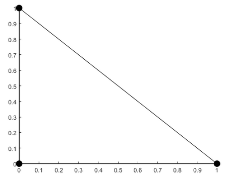
We first begin by creating a matrix with the coordinates, start at any node and go counter clockwise, we'll start in the 90 degree node, this is good practice.

P = [0 0
     1 0
     0 1]

Now we can visualize the element:

figure
patch(P(:,1),P(:,2),'w','FaceColor','none','DisplayName','Element'); hold on
plot(P(:,1),P(:,2),'ok','MarkerFaceColor','k','MarkerSize',10,'DisplayName','Nodes')
set(gca,'FontSize',14)
np = size(P,1);
xm = mean(P,1);
Tp = P+(xm-P)*0.2;
text(Tp(:,1),Tp(:,2),cellstr(num2str((1:np)')),'FontSize',14)

Now, we make the ansatz that the basis function for a linear triangle is

\varphi \left(\xi, \eta \right)=a_1 +a_2 \xi + a_3 \eta

We need to determine the three constants $a_1$ , $a_2$ and $a_3$ for a three noded element.

We use the definition of a basis function and create our system of equations for our case above where $\bm \xi \in \left\lbrack 0,1\right\rbrack$

\begin{array}{l} \varphi_1 \left(\xi_1, \eta_1 \right)=\varphi_1 \left(0,0\right)=a_1 +a_2\cdot 0+a_3\cdot 0=1\\ \varphi_1 \left(\xi_2, \eta_2 \right)=\varphi_1 \left(1,0\right)=a_1 +a_2\cdot 1+a_3\cdot 0=0\\ \varphi_1 \left(\xi_3, \eta_3 \right)=\varphi_1 \left(0,1\right)=a_1 +a_2\cdot 0+a_3\cdot 1=0 \end{array}

which leads to

\left\lbrack \begin{array}{ccc} 1 & 0 & 0\\ 1 & 1 & 0\\ 1 & 0 & 1 \end{array}\right\rbrack \left\lbrack \begin{array}{c} a_1 \\ a_2 \\ a_3 \end{array}\right\rbrack =\left\lbrack \begin{array}{c} 1\\ 0\\ 0 \end{array}\right\rbrack

\mathit{\mathbf{A} }\;\mathit{\mathbf{a} }=\mathit{\mathbf{b} }

\mathit{\mathbf{a} }={\mathit{\mathbf{A} } }^{-1} \mathit{\mathbf{b} }

and then

\varphi_1 \left(\xi, \eta \right)=\left\lbrack 1,\xi,\eta\right\rbrack \mathit{\mathbf{a} }

A = [1 0 0
     1 1 0
     1 0 1];
b = [1;0;0];
a = A\b

syms xi eta
phi_1(xi,eta) = [1, xi, eta]*a

1-\xi -\eta

But we can get all of the functions at the same time with

\mathit{\mathbf{A} }\;\mathit{\mathbf{C} }=\mathit{\mathbf{I} }

where

\mathit{\mathbf{C} }=\left\lbrack \begin{array}{ccc} a_{11} & a_{12} & a_{13} \\ a_{21} & a_{22} & a_{23} \\ a_{31} & a_{32} & a_{33} \end{array}\right\rbrack

C = A\eye(3)

C = 3x3    
     1     0     0
    -1     1     0
    -1     0     1

syms xi eta phi
phi(xi,eta) = [1, xi, eta]*C

\left(\begin{array}{ccc} 1-\xi -\eta & \xi & \eta \end{array}\right)

and we test the newly created function by evaluating it in the coordinates of our triangle:

phi(0,0)

\left(\begin{array}{ccc} 1 & 0 & 0 \end{array}\right)

phi(1,0)

\left(\begin{array}{ccc} 0 & 1 & 0 \end{array}\right)

phi(0,1)

\left(\begin{array}{ccc} 0 & 0 & 1 \end{array}\right)

Quadrilaterals or Bi-linear

The element coordinates

figure
patch(P(:,1),P(:,2),'w','FaceColor','none','DisplayName','Element'); hold on
plot(P(:,1),P(:,2),'ok','MarkerFaceColor','k','MarkerSize',10,'DisplayName','Nodes')
np = size(P,1);
xm = mean(P,1);
Tp = P+(xm-P)*0.2;
text(Tp(:,1),Tp(:,2),cellstr(num2str((1:np)')),'FontSize',14)
axis equal tight

Ansatz:

\varphi \left(\bm \xi \right)=a_1 +a_2 \xi+a_3 \eta+a_4 \xi \eta

A = [1 0 0 0
     1 1 0 0
     1 1 1 1
     1 0 1 0];
C = A\eye(4);
syms xi eta phi
phi(xi,eta) = simplify([1, xi, eta,xi*eta]*C)

\left(\begin{array}{cccc} {\left(\xi-1\right)}\,{\left(\eta-1\right)} & -\xi\,{\left(\eta-1\right)} & \xi\,\eta & -\eta\,{\left(\xi-1\right)} \end{array}\right)

matlabFunction(phi);
phi = @(xi,eta)[(xi-1.0).*(eta-1.0),-xi.*(eta-1.0),xi.*eta,-eta.*(xi-1.0)];

phi(P(:,1),P(:,2))

ans = 4x4    
     1     0     0     0
     0     1     0     0
     0     0     1     0
     0     0     0     1

Another way to get the same basis functions is by multiplying the one dimensional basis with the other:

\begin{array}{l} {\hat{\varphi} }_1 \left(\xi\right)=1-\xi\\ {\hat{\varphi} }_2 \left(\xi\right)=\xi \end{array}

\begin{array}{l} \varphi_1 \left(\xi,\eta\right)={\hat{\varphi} }_1 \left(\xi\right)\;{\hat{\varphi} }_1 \left(\eta\right)=\left(1-\xi\right)\left(1-\eta\right)\\ \varphi_2 \left(\xi,\eta\right)={\hat{\varphi} }_1 \left(\eta\right)\;{\hat{\varphi} }_2 \left(\xi\right)=\left(1-\eta\right)\xi\\ \varphi_3 \left(\xi,\eta\right)={\hat{\varphi} }_2 \left(\xi\right)\;{\hat{\varphi} }_2 \left(\eta\right)=\xi\;\eta\\ \varphi_3 \left(\xi,\eta\right)={\hat{\varphi} }_1 \left(\xi\right)\;{\hat{\varphi} }_2 \left(\eta\right)=\left(1-\xi\right)\eta \end{array}

This is why this element is refereed to as Bi-linear (Two linear). The same reasoning can be applied to get three dimensional basis functions, or tri-linear.

Triangular - quadratic

figure
patch(P(1:3,1),P(1:3,2),'w','FaceColor','none','DisplayName','Element'); hold on
plot(P(:,1),P(:,2),'ok','MarkerFaceColor','k','MarkerSize',8,'DisplayName','Nodes')
xlabel('\xi')
ylabel('\eta')
np = size(P,1);
xm = mean(P,1);
Tp = P+(xm-P)*0.2;
text(Tp(:,1),Tp(:,2),cellstr(num2str((1:np)')),'FontSize',14);
axis equal tight

Ansatz:

\varphi \left(\bm \xi \right)=a_1 +a_2 \xi+a_3 \eta+a_4 \xi^2 +a_5 \xi^{\;} \eta^{\;} +a_6 \eta^2

A = [1 0 0 0 0 0
     1 1 0 1 0 0
     1 0 1 0 0 1
     1 0.5 0 0.5^2 0 0
     1 0.5 0.5 0.5^2 0.5*0.5 0.5^2
     1 0 0.5 0 0 0.5^2];
C = A\eye(6);
syms xi eta phi
phi(xi,eta) = simplify([1, xi, eta xi^2 xi*eta eta^2]*C);

We'll use matlabFunction to get the numerical function for $\varphi$

simplify(phi).'

\left(\begin{array}{c} 2\,\eta^2 +4\,\eta \,\xi -3\,\eta +2\,\xi^2 -3\,\xi +1\\ \xi \,{\left(2\,\xi -1\right)}\\ \eta \,{\left(2\,\eta -1\right)}\\ -4\,\xi \,{\left(\eta +\xi -1\right)}\\ 4\,\eta \,\xi \\ -4\,\eta \,{\left(\eta +\xi -1\right)} \end{array}\right)

Bh = [diff(phi,xi)
      diff(phi,eta)]

\left(\begin{array}{cccccc} 4\,\eta +4\,\xi -3 & 4\,\xi -1 & 0 & 4-8\,\xi -4\,\eta & 4\,\eta & -4\,\eta \\ 4\,\eta +4\,\xi -3 & 0 & 4\,\eta -1 & -4\,\xi & 4\,\xi & 4-4\,\xi -8\,\eta \end{array}\right)

phi = matlabFunction(phi);

Bh = matlabFunction(Bh);

phi = @(xi,eta)[eta.*-3.0-xi.*3.0+eta.*xi.*4.0+eta.^2.*2.0+xi.^2.*2.0+1.0,xi.*(xi.*2.0-1.0),eta.*(eta.*2.0-1.0),xi.*(eta+xi-1.0).*-4.0,eta.*xi.*4.0,eta.*(eta+xi-1.0).*-4.0];
Bh =  @(xi,eta)reshape([eta.*4.0+xi.*4.0-3.0,eta.*4.0+xi.*4.0-3.0,xi.*4.0-1.0,0.0,0.0,eta.*4.0-1.0,eta.*-4.0-xi.*8.0+4.0,xi.*-4.0,eta.*4.0,xi.*4.0,eta.*-4.0,eta.*-8.0-xi.*4.0+4.0],[2,6]);

And we evaluate $\varphi$ in all the nodes to verify that it indeed is 1 in its node and 0 every where else

phi(P(:,1),P(:,2))

ans = 6x6    
     1     0     0     0     0     0
     0     1     0     0     0     0
     0     0     1     0     0     0
     0     0     0     1     0     0
     0     0     0     0     1     0
     0     0     0     0     0     1

OK!

Quadrilaterals - quadratic or bi-quadratic

figure
patch(P(1:4,1),P(1:4,2),'w','FaceColor','none','DisplayName','Element'); hold on
plot(P(:,1),P(:,2),'ok','MarkerFaceColor','k','MarkerSize',8,'DisplayName','Nodes')
xlabel('\xi')
ylabel('\eta')
np = size(P,1);
xm = mean(P,1);
Tp = P+(xm-P)*0.2;Tp(end,1) = Tp(end,1)+0.05;
text(Tp(:,1),Tp(:,2),cellstr(num2str((1:np)')),'FontSize',14)
axis equal tight

Ansatz:

\varphi \left(\mathit{\mathbf{\xi} }\right)=a_1 +a_2 \xi+a_3 \eta+a_4 \xi\;\eta+a_5 \xi^2 +a_6 \eta^2 +a_7 \xi^2 \eta+a_8 \xi\;\eta^{2\;} +a_9 \xi^2 \eta^2

A = [1 0 0 0 0 0 0 0 0
     1 1 0 0 1 0 0 0 0
     1 1 1 1 1 1 1 1 1
     1 0 1 0 0 1 0 0 0
     1 0.5 0 0 0.5^2 0 0 0 0
     1 1 0.5 0.5 1 0.5^2 0.5 0.5^2 0.5^2
     1 0.5 1 0.5 0.5^2 1 0.5^2 0.5 0.5^2
     1 0 0.5 0 0 0.5^2 0 0 0
     1 0.5 0.5 0.5^2 0.5^2 0.5^2 0.5^3 0.5^3 0.5^4];
C = A\eye(9);
syms xi eta phi
phi(xi,eta) = simplify([1, xi eta xi*eta xi^2 eta^2 xi^2*eta xi*eta^2 xi^2*eta^2]*C);
matlabFunction(phi);

phi = 
    @(xi,eta)[(eta.*-3.0+eta.^2.*2.0+1.0).*(xi.*-3.0+xi.^2.*2.0+1.0),xi.*(xi.*2.0-1.0).*(eta.*-3.0+eta.^2.*2.0+1.0),eta.*xi.*(eta.*2.0-1.0).*(xi.*2.0-1.0),eta.*(eta.*2.0-1.0).*(xi.*-3.0+xi.^2.*2.0+1.0),xi.*(xi-1.0).*(eta.*-3.0+eta.^2.*2.0+1.0).*-4.0,eta.*xi.*(xi.*2.0-1.0).*(eta-1.0).*-4.0,eta.*xi.*(eta.*2.0-1.0).*(xi-1.0).*-4.0,eta.*(eta-1.0).*(xi.*-3.0+xi.^2.*2.0+1.0).*-4.0,eta.*xi.*(eta-1.0).*(xi-1.0).*1.6e1]

Verify by evaluating all nodes!

phi(P(:,1),P(:,2))

ans = 9x9    
     1     0     0     0     0     0     0     0     0
     0     1     0     0     0     0     0     0     0
     0     0     1     0     0     0     0     0     0
     0     0     0     1     0     0     0     0     0
     0     0     0     0     1     0     0     0     0
     0     0     0     0     0     1     0     0     0
     0     0     0     0     0     0     1     0     0
     0     0     0     0     0     0     0     1     0
     0     0     0     0     0     0     0     0     1

OK!

Quadrilaterals - cubic or bi-cubic The coordinates to the nodes:

figure
patch(P(1:4,1),P(1:4,2),'w','FaceColor','none','DisplayName','Element'); hold on
plot(P(:,1),P(:,2),'ok','MarkerFaceColor','k','MarkerSize',5,'DisplayName','Nodes')
xlabel('\xi')
ylabel('\eta')
np = size(P,1);
xm = mean(P,1);
Tp = P+(xm-P)*0.1;
text(Tp(:,1),Tp(:,2),cellstr(num2str((1:np)')),'FontSize',14)
axis equal tight

Ansatz:

\varphi \left(\mathit{\mathbf{\xi} }\right)=a_1 +a_2 \xi+a_3 \eta+a_4 \xi\;\eta+a_5 \xi^2 +a_6 \eta^2 +a_7 \xi^2 \eta+a_8 \xi\;\eta^{2\;} +a_9 \xi^2 \eta^2 +a_{10} \xi^3 +a_{11} \eta^3 +a_{12} \xi^3 \eta+a_{13} \eta^3 \xi+a_{14} \xi^3 \eta^2 +a_{15} \eta^3 \xi^2 +a_{16} \xi^3 \eta^3

A = @(x,y)[1+x.*0 x y x.*y x.^2 y.^2 x.^2.*y x.*y.^2 x.^2.*y.^2 x.^3 y.^3 x.^3.*y y.^3.*x x.^3.*y.^2 y.^3.*x.^2 x.^3.*y.^3];
syms x y
S = sym(A(P(:,1),P(:,2)));
C = S\eye(16);
syms xi eta
phi = matlabFunction(simplify(A(xi,eta)*C));
phi = phi(xi,eta); % Wierd bug, needs to be substituted several times to be correct
phi = matlabFunction(phi)

phi = 
    @(eta,xi)[((eta.*1.1e+1-eta.^2.*1.8e+1+eta.^3.*9.0-2.0).*(xi.*1.1e+1-xi.^2.*1.8e+1+xi.^3.*9.0-2.0))./4.0,eta.*(eta.*-9.0+eta.^2.*9.0+2.0).*(xi.*1.1e+1-xi.^2.*1.8e+1+xi.^3.*9.0-2.0).*(-1.0./4.0),(eta.*xi.*(eta.*-9.0+eta.^2.*9.0+2.0).*(xi.*-9.0+xi.^2.*9.0+2.0))./4.0,xi.*(xi.*-9.0+xi.^2.*9.0+2.0).*(eta.*1.1e+1-eta.^2.*1.8e+1+eta.^3.*9.0-2.0).*(-1.0./4.0),eta.*(eta.*-5.0+eta.^2.*3.0+2.0).*(xi.*1.1e+1-xi.^2.*1.8e+1+xi.^3.*9.0-2.0).*(-9.0./4.0),eta.*(eta.*-4.0+eta.^2.*3.0+1.0).*(xi.*1.1e+1-xi.^2.*1.8e+1+xi.^3.*9.0-2.0).*(9.0./4.0),eta.*xi.*(eta.*-9.0+eta.^2.*9.0+2.0).*(xi.*-5.0+xi.^2.*3.0+2.0).*(9.0./4.0),eta.*xi.*(eta.*-9.0+eta.^2.*9.0+2.0).*(xi.*-4.0+xi.^2.*3.0+1.0).*(-9.0./4.0),eta.*xi.*(eta.*-4.0+eta.^2.*3.0+1.0).*(xi.*-9.0+xi.^2.*9.0+2.0).*(-9.0./4.0),eta.*xi.*(eta.*-5.0+eta.^2.*3.0+2.0).*(xi.*-9.0+xi.^2.*9.0+2.0).*(9.0./4.0),xi.*(xi.*-4.0+xi.^2.*3.0+1.0).*(eta.*1.1e+1-eta.^2.*1.8e+1+eta.^3.*9.0-2.0).*(9.0./4.0),xi.*(xi.*-5.0+xi.^2.*3.0+2.0).*(eta.*1.1e+1-eta.^2.*1.8e+1+eta.^3.*9.0-2.0).*(-9.0./4.0),eta.*xi.*(eta.*-5.0+eta.^2.*3.0+2.0).*(xi.*-5.0+xi.^2.*3.0+2.0).*(8.1e+1./4.0),eta.*xi.*(eta.*-4.0+eta.^2.*3.0+1.0).*(xi.*-5.0+xi.^2.*3.0+2.0).*(-8.1e+1./4.0),eta.*xi.*(eta.*-4.0+eta.^2.*3.0+1.0).*(xi.*-4.0+xi.^2.*3.0+1.0).*(8.1e+1./4.0),eta.*xi.*(eta.*-5.0+eta.^2.*3.0+2.0).*(xi.*-4.0+xi.^2.*3.0+1.0).*(-8.1e+1./4.0)]

Basic FEM

Defining basis function in 2D

Triangular elements

Quadrilaterals or Bi-linear

Triangular - quadratic

Quadrilaterals - quadratic or bi-quadratic