Download this page as a Matlab LiveScript
Table of contents
Solve the following differential equation using numerical integration
Recall: integration points integrate polynomials of degree exactly!
Draw the mesh, schematically, number the nodes, put down the boundary conditions.
Choose the approximation, i.e., element type. This defines the mesh and the basis functions as well as the Gauss integration order for the matrices.
clear
syms ue(x)
DE = -2*diff(ue,x,2) - ue == x^2;
du = diff(ue,x);

BC = [du(-1)==2, ue(5)==3];

ue = dsolve(DE, BC);

figure
fplot(ue,[-1,5], 'r', 'LineWidth',2)
Solve numerically using N quadratic elements
N = 2;
nnod = N*2+1; % Number of nodes
neq = nnod*1; % Number of equations, one degree of freedom per node
xnod = linspace(-1,5,nnod);
Visualizing the mesh
figure
plot(xnod, xnod*0, 'ok', MarkerFaceColor='k',MarkerSize=15)
text(xnod-0.03, xnod*0, cellstr(num2str([1:nnod]')), Color='w')
axis equal tight
ylim([-0.5,0.5]); box off
Define the mesh topology, i.e., node connectivity
nodes = [(1:2:nnod-2)', (2:2:nnod-1)', (3:2:nnod)'];Basis functions are defined here as anonymous functions. These are numeric and evaluate very fast compared to symbolic functions.
phi = @(xi)[(xi.*2.0-2.0).*(xi-1.0./2.0),xi.*(xi-1.0).*-4.0,xi.*(xi-1.0./2.0).*2.0];
dphi = @(xi)[xi.*4.0-3.0,xi.*-8.0+4.0,xi.*4.0-1.0];
The Gauss order is choosen, here, it is choosen by the highest polynomial order in the differential equation.
order = 4;
[gp, gw] = gauss(order, 0, 1);
We pre-allocate variables to their final sizes, this is done for execution performance. There are faster methods of doing this, but for readability, we will stick to this. Ask Mirza if interested for more info on performance optimization.
S = zeros(neq,neq);
M = S;
F = zeros(neq,1);
The main assembly loop. The heart of any FEM solver. We are looping over all elements to compute the element stiffness, mass and load matrices.
The internal loop is the Gauss integration loop.
remember is the length (or size) of the parameter space!
where
for iel = 1:N
    inod = nodes(iel,:);
    xc = xnod(inod);
    h = xc(end)-xc(1);
    Se = zeros(3,3);
    Me = Se;
    fe = zeros(3,1);
    for ig = 1:length(gp)
        xi = gp(ig);
        iw = gw(ig);

        Se = Se + 2*dphi(xi)'*dphi(xi)*1/h*1*iw;
        Me = Me + phi(xi)'*phi(xi)*h*1*iw;

        x = phi(xi)*xc';
        fe = fe + phi(xi)' * x^2 * h * 1 * iw;
    end
    % Assembly
    S(inod,inod) = S(inod, inod) + Se;
    M(inod,inod) = M(inod, inod) + Me;
    F(inod) = F(inod) + fe;
end
S = S-M;
Boundary conditions
g = zeros(neq,1);
g(1) = -2*2;

alldofs = 1:neq;
presc = alldofs(end); %u is known in the last degree of freedom
u = zeros(neq,1); %Pre-allocate
u(presc) = 3; %prescribe
free  = setdiff(alldofs,presc);
Modify the right hand side, e.g.,
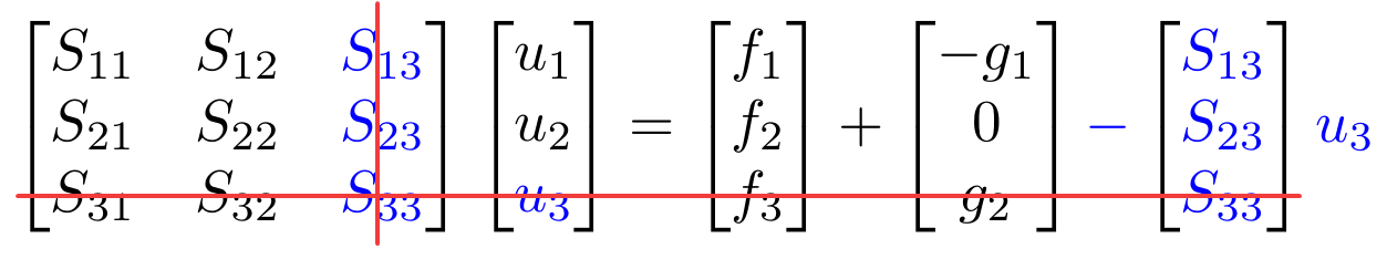
F = F + g - S(:, presc)*u(presc);Reduce the system and solve
u(free) = S(free,free)\F(free);figure
fplot(ue,[-1,5], 'r', 'LineWidth',2)
hold on
plot(xnod, u, 'bo')
The blue dots represent the solution variables.
Every quadratic element is defined by three nodal values and in between we need to interpolate using the quadratic basis functions.
For every element the approximation is given by:
figure
fplot(ue,[-1,5], 'r', 'LineWidth',2)
hold on
plot(xnod, u, 'bo')We will let be a set of evenly spaced numbers between 0 and 1.
for iel = 1:N
    iel
    inod = nodes(iel,:);
    xc = xnod(inod);
    U = u(inod);
    xi = linspace(0,1,100)';

    Ue = phi(xi)*U;
    Xe = phi(xi)*xc';
    plot(Xe,Ue,'-')
endtitle("Two quadratic elements")
Now we want to compute the difference between the function for each element and adding it all up.
where
remember:
ue = matlabFunction(ue);

L2err = 0;
for iel = 1:N
    inod = nodes(iel,:);
    xc = xnod(inod);
    h = xc(end)-xc(1);
    U = u(inod);
    err = 0;
    for ig = 1:length(gp)
        xi = gp(ig);
        iw = gw(ig);
        x = phi(xi)*xc';
        Ue = phi(xi)*U;
        err = err + (ue(x)-Ue)^2 * h * 1 * iw;
    end
    L2err = L2err + err;
end
L2err = sqrt(L2err)
L2err = 9.4298We shall now compute the error for elements and plot the convergence.
clear

syms ue(x)
DE = -2*diff(ue,x,2) - ue == x^2;
du = diff(ue,x);
BC = [du(-1)==2, ue(5)==3];
ue = dsolve(DE, BC);

NN = [2,4,8,16,32,64,128];
L2Err1 = []; Time1 = []; XX1 = [];
L2Err2 = []; Time2 = []; XX2 = [];
To keep the code somewhat clean, we shall move the whole solver code into a function called FEM1DLinSolver.
for N = NN
    tic
    [u,L2err,h,xnod] = MyKickassQuadSolver(N,ue);
    Time1(end+1) = toc;
    L2Err1(end+1) = L2err;
    XX1(end+1)=h;

    figure(1); clf; hold on
    fplot(ue,[-1,5],'r')
    plot(xnod,u,'bo')
    title(sprintf("%d quadratic elements",N))

    tic
    [u,L2err,h,xnod] = MyKickassLinSolver(N,ue);
    Time2(end+1) = toc;
    L2Err2(end+1) = L2err;
    XX2(end+1)=h;

    figure(2); clf; hold on
    fplot(ue,[-1,5],'r')
    plot(xnod,u,'bo-')
    title(sprintf("%d linear elements",N))
end

figure; hold on
plot(NN,L2Err1,'-ro','DisplayName','Quadratic Approximation')
plot(NN,L2Err2,'-bs','DisplayName','Linear Approximation')
set(gca,'XScale','log','YScale','log')
grid on
xticks(NN)
axis equal
xlabel("Number of elements"); ylabel("L_2 error")
legend("show","Location","southwest")
Not only is the quadratic approximation better for every number of elements, it also converges faster than the linear approximation.

Note that evaluating runtime for these small problems is tricky, a definitive comparison can only be seen with a high number of elements, since the overhead of the computations is significant when we have a small number of elements.

It makes more sense to plot the number of degrees of freedom than number of elements.
To do a proper convergence analysis we shall plot the errors vs the mesh size, rather than number of degrees of freedom or number of elements. We can then compute the slope of the convergence graph, which is the rate of convergence. It can be mathematically shown what convergence rate we can expect from a certain interpolant using error estimation.
To compute the convergence rate, we can do a numerical convergence study by computing a number of errors, each time doubling the number of elements. The convergence rate is then given by
where is the mesh size.

The slope of the error convergence for the quadratic approximation tends towards 3 and for the linear approximation towards 2.
diff(log(L2Err1))./diff(log(XX1))ans = 1x6
3.2776 3.4207 3.1950 3.0607 3.0162 3.0041diff(log(L2Err2))./diff(log(XX2))ans = 1x6
0.9803 1.5597 1.8643 1.9639 1.9908 1.9977function [u,L2err,h,xnod] = MyKickassQuadSolver(N,ue)
nnod = N*2+1;
xnod = linspace(-1,5,nnod);
nodes = [(1:2:nnod-2)', (2:2:nnod-1)', (3:2:nnod)'];
neq = nnod*1;
phi = @(xi)[(xi.*2.0-2.0).*(xi-1.0./2.0),xi.*(xi-1.0).*-4.0,xi.*(xi-1.0./2.0).*2.0];
dphi = @(xi)[xi.*4.0-3.0,xi.*-8.0+4.0,xi.*4.0-1.0];
order = 4;
[gp, gw] = gauss(order, 0, 1);
S = zeros(neq,neq);
M = S;
F = zeros(neq,1);
for iel = 1:N
inod = nodes(iel,:);
xc = xnod(inod);
h = xc(end)-xc(1);
Se = zeros(3,3);
Me = Se;
fe = zeros(3,1);
for ig = 1:length(gp)
xi = gp(ig);
iw = gw(ig);
Se = Se + 2*dphi(xi)'*dphi(xi)*1/h*1*iw;
Me = Me + phi(xi)'*phi(xi)*h*1*iw;
x = phi(xi)*xc';
fe = fe + phi(xi)' * x^2 * h * 1 * iw;
end
% Assembly
S(inod,inod) = S(inod, inod) + Se;
M(inod,inod) = M(inod, inod) + Me;
F(inod) = F(inod) + fe;
end
S = S-M;
g = zeros(neq,1);
g(1) = -2*2;
alldofs = 1:neq;
presc = alldofs(end);
u = zeros(neq,1);
u(presc) = 3;
free = setdiff(alldofs,presc);
F = F + g - S(:, presc)*u(presc);
u(free) = S(free,free)\F(free);
ue = matlabFunction(ue);
L2err = 0;
for iel = 1:N
inod = nodes(iel,:);
xc = xnod(inod);
h = xc(end)-xc(1);
U = u(inod);
err = 0;
for ig = 1:length(gp)
xi = gp(ig);
iw = gw(ig);
x = phi(xi)*xc';
Ue = phi(xi)*U;
err = err + (ue(x)-Ue)^2 * h * 1 * iw;
end
L2err = L2err + err;
end
L2err = sqrt(L2err);
endfunction [u,L2err,h, xnod] = MyKickassLinSolver(N,ue)
xnod = linspace(-1,5,N+1);
nodes = [(1:N)', (2:N+1)'];
nnod = length(xnod);
neq = nnod*1;
phi = @(xi)[1-xi, xi];
dphi = [-1, 1];
order = 2;
[gp, gw] = gauss(order, 0, 1);
S = zeros(neq,neq);
M = S;
F = zeros(neq,1);
for iel = 1:N
inod = nodes(iel,:);
xc = xnod(inod);
h = xc(end)-xc(1);
Se = zeros(2,2);
Me = Se;
fe = zeros(2,1);
for ig = 1:length(gp)
xi = gp(ig);
iw = gw(ig);
Se = Se + 2*dphi'*dphi*1/h*1*iw;
Me = Me + phi(xi)'*phi(xi)*h*1*iw;
x = phi(xi)*xc';
fe = fe + phi(xi)' * x^2 * h * 1 * iw;
end
% Assembly
S(inod,inod) = S(inod, inod) + Se;
M(inod,inod) = M(inod, inod) + Me;
F(inod) = F(inod) + fe;
end
S = S-M;
g = zeros(neq,1);
g(1) = -2*2;
alldofs = 1:neq;
presc = alldofs(end);
u = zeros(neq,1);
u(presc) = 3;
free = setdiff(alldofs,presc);
F = F + g - S(:, presc)*u(presc);
u(free) = S(free,free)\F(free);
ue = matlabFunction(ue);
L2err = 0;
for iel = 1:N
inod = nodes(iel,:);
xc = xnod(inod);
h = xc(end)-xc(1);
U = u(inod);
err = 0;
for ig = 1:length(gp)
xi = gp(ig);
iw = gw(ig);
x = phi(xi)*xc';
Ue = phi(xi)*U;
err = err + (ue(x)-Ue)^2 * h * 1 * iw;
end
L2err = L2err + err;
end
L2err = sqrt(L2err);
endfunction [x, w, A] = gauss(n, a, b)
%------------------------------------------------------------------------------
% gauss.m
%------------------------------------------------------------------------------
%
% Purpose:
%
% Generates abscissas and weigths on I = [ a, b ] (for Gaussian quadrature).
%
%
% Syntax:
%
% [x, w, A] = gauss(n, a, b);
%
%
% Input:
%
% n integer Number of quadrature points.
% a real Left endpoint of interval.
% b real Right endpoint of interval.
%
%
% Output:
%
% x real Quadrature points.
% w real Weigths.
% A real Area of domain.
%------------------------------------------------------------------------------
% 3-term recurrence coefficients:
n = 1:(n - 1);
beta = 1 ./ sqrt(4 - 1 ./ (n .* n));
% Jacobi matrix:
J = diag(beta, 1) + diag(beta, -1);
% Eigenvalue decomposition:
%
% e-values are used for abscissas, whereas e-vectors determine weights.
%
[V, D] = eig(J);
x = diag(D);
% Size of domain:
A = b - a;
% Change of interval:
%
% Initally we have I0 = [ -1, 1 ]; now one gets I = [ a, b ] instead.
%
% The abscissas are Legendre points.
%
if ~(a == -1 && b == 1)
x = 0.5 * A * x + 0.5 * (b + a);
end
% Weigths:
w = V(1, :) .* V(1, :);
w = w';
x=x';
end