Before approximating solutions to differential equations we shall introduce the concept and method on a simpler problem:
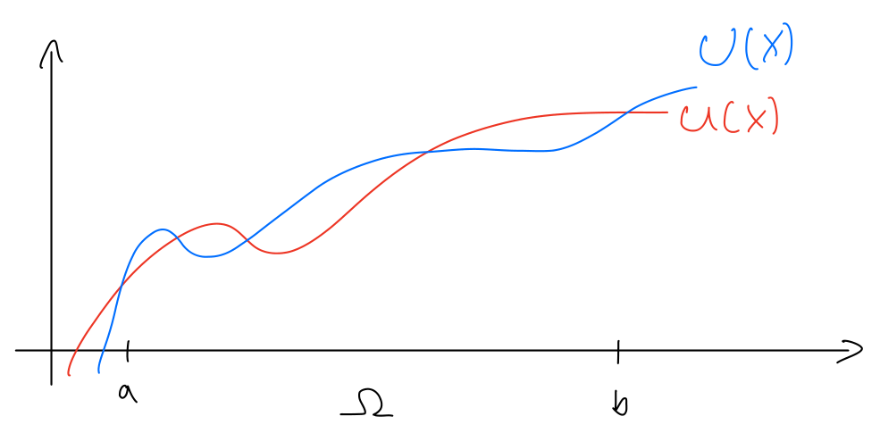
Given a polynomial function U(x) of some order, find the best approximation to some target function u(x) in the range x∈[a,b]
So u(x) is a known function and we need to find another function U(x) in the given range to approximate u.
First we need to define what is meant with "finding an approximation".
Given that U(x) is a polynomial function of some order we have the following choices to make (degrees of freedom):
We need to chose the polynomial order
We need to choose the constants of the polynomial function
We can define the polynomial function as e.g.,
U(x)=a1+a2x+a3x2
which is a second order polynomial where ai are the constants to be tweaked to find the best approximation to u(x). More generally we can say that the approximation function is defined as
U(x)=i=1∑naixi−1
where n−1 defines the order of the polynomial and we need to find the constants a1,⋯,ai,⋯,an which give the best approximation.
We can also choose to define U as linear combinations of basis functions using control points ui:
The control point always lie on the function U and we shall see that this has more advantages when we get to later topics.
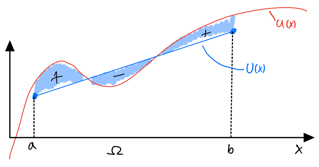
Now, what does "best approximation" mean? Well, there can be many definitions, but we shall look at it as finding the parameters ui such that the area between the curves is as little as possible. This is equivalent to saying that on average the error between the functions is 0. Now, let's address the obvious: If we know u, why not just choose the same polynomial or a very high polynomial? The answer is: We do not know what u is in general, this exercise here is just to illustrate the method which, as we shall see, also works the same for approximating solutions to differential equations. Besides, choosing a high polynomial as an approximation comes with computational cost and other numerical problems, there are better ways of achieving higher accuracy as we shall see.
Example
Let the approximation be linear, basically a linear interpolation between the nodal values u1 and u2
U(x)=u1φ1b−ab−x+u2φ2b−ax−a
φi(x) are called basis functions and are Lagrange Polynomials which are used in a type of interpolation called Lagrange Interpolation. We prefer this type of interpolation because ui become points on the approximation curve.
⚠ Note
We shall later see how the basis functions φi are defined and learn about their properties.
To define an average area between the curves we first define the difference between the curves, a.k.a the residual: r(x,ui)=U(x,ui)−u(x)
Now our problem becomes on the form: Find ui such that we minimize the residual r(x,ui)=U(x)−u(x) on the domain x∈[a,b]
This is equivalent to minimizing the area between the curves and we can formulate
Minimizing the area A in (5) means finding which ui minimize it. This method is called the weighted residual method, and the w(x) in the equation is the weight function for which there are several choices.
The Ritz method is a weighted residual method and aims at minimizing the square of the residual. The Ritz method was suggested by the Austrian physicist W. Ritz as a way of obtaining approximate solutions to physical problems fulfilling a minimum principle [3]. Lord Rayleigh published an article claiming that Ritz's idea was already presented in his own prior work, leading to the name Rayleigh-Ritz for this method, used by many authors even to this day. Although it has been shown clearly in [2] that Rayleigh's claim is not justified.
The Ritz method suggests to approximate the actual solution u by a given function U on the form
u(x)≈U(x)=i=0∑naixi
which then shall minimize the functional
S(ai)=21∫abr2(x,ai)dx
with respect to the parameters ai.
This is minimized by setting the partial derivatives to zero
∂ai∂S=0⇒ai
which leads to a system of equations to solve for the parameters ai.
If we instead use the form
u(x)≈U(x)=i=0∑nuiφ(x)
with φ1=x,φ2=x2,etc. we can get the weight function by
We have not been introduced to the Ritz method in the proper setting (which is what it initially was used for); applied on a minimum principle for solving problems consisting of differential equations, see e.g., [4] for an historical overview of the method and how it led up to the modern method we now know as the finite element method. Thus consider the differential equation
dxd(kdxdu)=fon x∈[0,1]
with u(0)=0 and dxdu(1)=0. Now, set k=1 and f=1. Let u≈U(x)=u1φ1(x)+u2φ2(x) with φ1(x)=x and φ2(x)=x2. The exact solution to this problem is u(x)=x−x2/2, so the approximation has a form which contains the exact solution. Now, there exists a minimization principle of (14) such that we minimize the functional
S(u1,u2)=21∫01(dxdU)2dx−∫01Udx
This is a variational form of (14) and represents the potential energy of the physical system which (14) models. The solution u to the problem in (14) is the one that minimizes the potential energy in (15). The potential energy is minimized by differentiating the functional with respect to the parameters, u1 and u2 and setting the derivatives to zero. We will first differentiate and arrive at
and thus u1=1 and u2=−1/2 and subsequently U(x)=x−x2/2=u(x).
This method can be generalized to use an arbitrary number of approximating functions for a problem which can be written as a variational form or a minimization principle. We summarize the method in general terms, let the approximation have the form
u(x)≈U(x)=i=1∑nuiφi(x)
where ui are the unknown parameters to be determined by the method and φi(x) are known functions, typically simple polynomials of trigonometric function chosen cleverly to approximate the differential equation well. The Ritz's method minimizes the functional S by only using functions of the specific form (18), which is straight forward since now the functional is a function of the parameters ui:
S(U)=S(i=1∑nuiφi(x))
and the minimum is obtained by differentiating S with respect to ui and setting the derivative to zero, leading to n equation to be solved for the unknown parameters ui. For our model problem (as an example) we have
as long as we have non-trivial solutions away from the boundary, i.e., U=0, recall that the boundary conditions state U(0)=0 and dxdU(1)=0. The positive definiteness guarantees that S is non-singular, and thus that the system Su=f has a unique solution. The fact that the stiffness matrix is symmetric, positive definitive and non singular is a cornerstone of an efficient numerical method and characteristic for the finite element method.
The strength of the Ritz method lies in that it recovers the optimal solution for the parameters ui, since it is based on the minimum of potential energy principle and thus any other choice of ui will take us away from the minimum of potential energy. Additionally, if the exact solution is contained in the approximation, we are certain to recover it using the method. This is however, not the case in general, especially in several dimensions, we can only get an approximation of the solution which is in a sense optimal on average.
The method which Ritz proposed was almost immediately utilized by soviet engineers, such as Timoshenko who first realized the importance of the method for engineering applications and used the method on many interesting problems [5]. Then Ivan Bubnov discovered the method from Timoshenko and used it on shell computations for ship (and submarine) building [6] leading to a manual on ship building with a heavy use of the Ritz method. Bubnov contributed to the development of the finite element method by realizing in [7] that simple approximate solutions could be obtained by multiplying the differential equation by φi and integrate over the entire domain to obtain the same equations that Timoshenko found (Bubnov did not cite the work of Ritz directly). Bubnov's realization gave the recipe for deriving the weak form and deriving the linear system without needing a principle of minimum potential energy as is the case with the Ritz method.
In 1915, the soviet engineer Boris G. Galerkin (more accurately Galyorkin), suggested a variation of the Ritz method in his most famous publication [1], which is usually quoted when referring to the Galerkin method. Galerkin's main contribution in that paper was to realize that the minimization principle is not needed in order to construct a finite-dimensional system following the recipe by Bubnov. It is noteworthy that Galerkin did refer to this method as the Ritz method. Providing many examples from application maybe is an explanation for why we today know this as a Galerkin method instead of the Ritz method.
Galerkin's method suggests, instead of differentiating r(x,ui) in (5), we differentiate the approximation U(x,ui) with respect to the parameters ui
Considering the same model problem from (14), we multiply the equation by v and integrated over the whole domain by parts to get
∫01kdxdudxdvdx=∫01fvdx
Galerkin suggested that given that the trial function or approximation has the form U(x)=∑i=1nuiφi(x), the weight function v should have the same form as the trial function, i.e., v(x)=∑i=1nciφi(x), meaning we should simply choose the basis functions as the weight functions, and loosely speaking, setting v=φj, and in the case of the weak form the derivative of the basis weight function become dxdv=dxdφj such that the weak form in (34) becomes:
∫abkdxdUdxdφjdx=∫abfφjdx
which is the same expression obtained using the Ritz method! This holds in a much more general setting but much more importantly: the Galerkin method can be used even if no minimum principle exists. It is always possible to take a general (partial) differential equation and multiply by a test function, integrate over the entire domain (using partial integration) to obtain a Galerkin method. The real strength of Galerkin's method is in its minimization properties (and thus the relation to Ritz' method).
Example: Find an approximate solution to the differential equation
dx2d2u+2dxdu=xfor x∈[0,1]
with the boundary conditions u(0)=u(1)=0.
It is possible to show that there is no corresponding minimum principle in the sense we have discussed earlier, and thus Ritz' method cannot be applied. The exact solution to this equation is given by u=x(x−1)/4, and we use the approximation U=ax(x−1). A weak form can be derived using the recipe of multiplying by v and integrating by parts to get
∫01−dxdudxdv+2dxduvdx=∫01xvdx∀v such that v=0 where u is known.
Applying Galerkin's method means using v=∂a∂U=x(x−1), so we obtain
Above we mentioned the minimization properties of Galerkin's method. Let us explore what this means and how Galerkin's method relates to minimization, least squares and orthogonality. For a great visual proof that inspired this text see this video by Virtually Passed. Another great explanation of the Galerkin method with special emphasis on the orthogonality is this video by Good Vibrations with Freeball
The least squares method is about minimizing the squared distance of a set of functional values g(xj) to an approximation of g(x)
g(x)≈G(x)=i=1∑naiϕi(x),
where ai are the unknown parameters to be decided and ϕi(x) are known functions. In other words, we are trying to fit an approximation U(x,ai) to a set of points g(xj). The reader might remember that in the discrete least squares method one minimizes the squares of the difference point-wise:
aiminj=1∑mr(xj,ai)2,
where
r(xj,ai)=G(xj,ai)−g(xj)
One way of getting to the solution and find the parameters ai that minimize the residual is using calculus, we remember that taking the derivative and setting it to zero leads to the minimum. We denote the squared residual
which is a system of n equations where we solve for ai. This can be written using matrices to express the equation as a linear system which can be solved more efficient, also using some linear algebra we can show the orthogonality more intuitively by using geometric relations.
We notice that rj=a1ϕ1(xj)+a2ϕ2(xj)+...+anϕn(xj)−g(xj), which we can write as
from this we recognize the transpose of A and thus we can have
ATr=0
inserting r=Ax−g into this we get
AT(Ax−g)⇒=0ATAx=ATg
from which we get the components ai by
x=(ATA)−1ATg
If we use linear approximation U(x)=a1ϕ1(x)+a2ϕ2(x) we have ϕ1(x)=1−x and ϕ2(x)=x. Which would yield an m−by−2A matrix where m is the number of data points to fit the approximation to.
Now that the matrix formulation is introduced we can formulate the problem differently: Find the vector x such that
min∣∣Ax−g∣∣2
which can be accomplished by making the approximation Ax as close to g as possible. For any non-zero choice of x, the transformation by A will make the approximation adhere to a plane, a so called column space of A. Recall that the matrix A is made up by functions ϕi=[ϕi(x1),ϕi(x2),...,ϕi(xm)]T such that
A=[ϕ1ϕ2⋯ϕn]m×n
which means that for any choice of ai the resulting vector Ax=a1ϕ1+a2ϕ2+... will always be parallel to the vectors ϕi.
We can exemplify the functions ϕi(x) as basis functions which span a plane (see the figure) onto which the approximation U(x) must be confined. For any point gi a shortest distance to the solution plane is obviously an orthogonal projection as is clear from the figure. This means that the optimal choice of ai will lead to the residual error vector r being orthogonal to the basis functions ϕ. Let x∗ denote the optimal parameters ai such that the approximation vector becomes U=Ax∗ and from the figure we see that
r=g−Ax∗⊥ϕ1⊥ϕ2
since
ϕi⋅(g−Ax∗)=0
but we can express this scalar product as a matrix multiplication
ϕi⋅(g−Ax∗)=AT(g−Ax∗)=0
from which we get
ATAx∗=⇒ATgx∗=(ATA)−1ATg
This discrete setting can be generalized into a continuous setting, where we have functions instead of vectors and integrals instead of finite sums. The functions u and v are orthogonal when the integral of their product is zero, i.e.,
∫f(x)g(x)dx=0
this is equivalent of a scalar product. This, so called Galerkin orthogonality is the central idea of the Galerkin method and what Galerkin discovered. This orthogonality concept is what connects to the least squares method, to minimization and to Ritz and to variational calculus.
∫r(x,ui)φj(x)dx=0
The residual function r(x,ui) is orthogonal to the basis function φj if the above integral holds. From this we find ui which minimizes the residual error and any deviation from these will increase the residual error.
We want to approximate the function u using a linear function U
U(x)=φ1(x)u1+φ2u2=u11−01−x+u21−0x−0
Thus φ1=1−x, φ2=x
We want to determine the function U(x) that minimizes the area between U(x) and u(x). Using the Galerkin method this means finding u1 and u2 such that
Choosing the approximation u≈U=u1φ1+u2φ2 is not the only option- We can increase the polynomial order by adding terms to get quadratic, cubic and even higher order approximations.
We will spend a whole section on studying how to define and create basis functions φi later. For now let us take a closer look at the quadratic approximation.
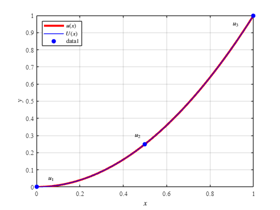
We want to approximate u=x2 using quadratic basis functions on the interval 0≤x≤1 for which we have the basis functions to be
φ1φ2φ3=2(x−1)(x−1/2)=−4x(x−1)=2x(x−1/2)
and our approximation becomes
u(x)≈U(x)=i=1∑3uiφi(x)
Using Galerkin, we get 3 equations:
∫01(U−ui)φidx=0for i=1,2,3
3 equations and 3 unknowns ⇒ unique solution.
clear; close all
syms x u1 u2 u3
The quadratic basis function is defined for x∈[0,1]
If we take a look at the function u(x)=2xsin(2πx)+3 for x in 0≤x≤1
We can see from the graph that a linear approximation or even a quadratic approximation will not be able to "approximate" this exactly! In general, even with higher and higher polynomials we would not be able to exactly approximate sinusoids... on the whole domain. Instead of trying to fit one function across the whole domain, we can approximate smaller pieces of it by just limiting the approximation to a set of subdomains. This is called piecewise approximation. We essentially divide the domain into finite elements.
For x∈[x1,x2], let a=x1 and b=x2
Using linear basis functions be have
φ=[b−ab−x,b−ax−a]
Then we let x∈[x2,x3] and a=x2, b=x3, etc
1: The Finite Element Method
In the next section, we will see how this method is derived and implemented in Matlab.
B.
G. Galerkin, “Series occurring in various questions concerning the
elastic equilibrium of rods and plates,”Vestnik Inzhenerov i
Tekhnikov, (Engineers and Technologists Bulletin), vol. Vol. 19,
pp. 897–908, 1915.
[2]
A.
W. Leissa, “The historical bases of the rayleigh and ritz
methods,”Journal of Sound and Vibration, vol. 287, no.
4, pp. 961–978, 2005, doi: https://doi.org/10.1016/j.jsv.2004.12.021.
[3]
W.
Ritz, “Über eine neue methode zur lösung gewisser
variationsprobleme der mathematischen physik.” vol. 1909, no.
135, pp. 1–61, 1909, doi: doi:10.1515/crll.1909.135.1.
[4]
M.
J. Gander and G. Wanner, “From euler, ritz, and galerkin to modern
computing,”SIAM Review, vol. 54, no. 4, pp. 627–666,
2012, doi: 10.1137/100804036.
[5]
S.
P. Timoshenko, Sur la stabilité des systèmes élastiques. A.
Dumas, 1914, pp. 496–566.
[6]
I.
G. Bubnov, “Structural mechanics of shipbuilding,”
1914.
[7]
I.
G. Bubnov, “Report on the works of professor timoshenko which were
awarded the zhuranskyi prize,”Symposium of the Institute of
Communication Engineers, 1913.