Table of contents

Interpolation in 2D

Interpolating from nodal values. Give som field in the nodal values of an element we can compute values somewhere inside the element using the basis functions as an interpolant. This section shows how to do this and how the choice of basis functions effect the interpolation accuracy.

Bi-linear interpolation

Given some element in 2D

P = [0   0
     1.0   0
     0.9  1.0
     -0.1,  1.2];

We have some discrete scalar field in the nodes $\bf P$ given by $\bf U$

U = [20
     30
     40
     25];

We can visualize this by

figure
patch("Faces",[1,2,3,4],'Vertices', P, 'CData', U, 'FaceColor', 'interp')
hold on; axis equal tight; colormap jet; colorbar
plot(P(:,1), P(:,2),'ok','MarkerFaceColor','k')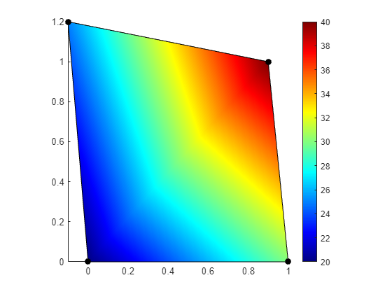

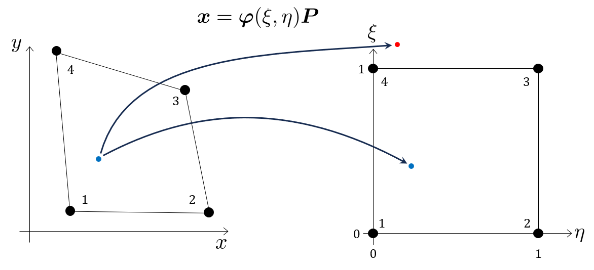
Now we want to know what the value $u_h$ is in the point $\left(x,y\right)$.

We can use the basis functions for a four-noded quadliteral element to interpolate the nodal values. See how to derive basis functions or just grab the pre-computed basis functions. We have, for the element above, the basis functions defined for the parametric coordinates $\xi ,\eta \in \left\lbrack 0,1\right\rbrack$

phi = @(xi,eta)[(eta-1.0).*(xi-1.0),-xi.*(eta-1.0),eta.*xi,-eta.*(xi-1.0)];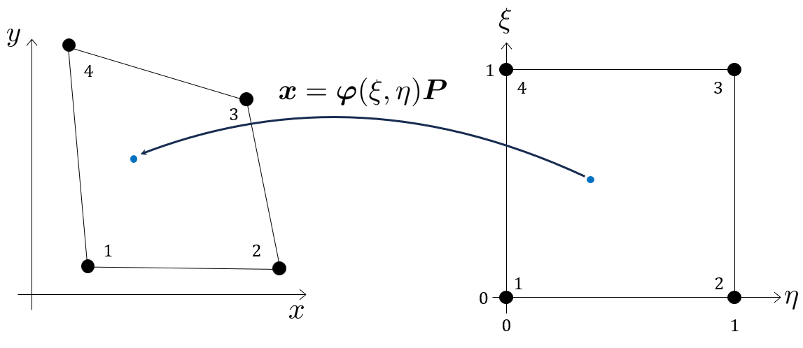

Now, we can easily interpolate $u_h$ using parametric coordinates by $u_h \left(\xi ,\eta \right)= \bm \varphi \left(\xi ,\eta \right) \bf P$

syms xi eta 
Uh = phi(xi, eta)*U; 
Uh = simplify(Uh)

E.g., in the midpoint we have $u_h \left(\xi =0\ldotp 5,\eta =0\ldotp 5\right)$

double(subs(Uh,[xi,eta],[0.5,0.5]))

ans = 28.7500

The issue is when we actually want the values $u_h$ as functions of the coordinates $x,y$, i.e., $u(x,y)$, we need to solve a system of equations which, depending on the geometry of the element (the coordinates $\bf P$), will be either linear or non-linear. For instance when $\bf P$ is affine:

P = [0    0
     2.0  0
     2.0  1.0
     0,   1];

figure
patch("Faces",[1,2,3,4],'Vertices', P, 'FaceColor', 'w')
hold on; axis equal tight;
plot(P(:,1), P(:,2),'ok','MarkerFaceColor','k')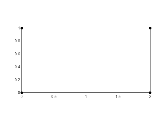

We want to solve $\bm{\varphi} \left(\xi ,\eta \right) \mathbf P = \left\lbrack x, y\right\rbrack$ for $\xi \left(x,y\right)$ and $\eta \left(x,y\right)$

syms x y
eqs = phi(xi, eta)*P == [x y];
eqs = simplify(eqs)

we see that this is trivial

[xi, eta] = solve(eqs,[xi,eta])

we can then substitute this into $\bm \varphi(\xi, \eta)$ to get $\bm \varphi \left(x,y\right)$

simplify(phi(xi,eta))

which we can use as an interpolant to get

If, however, the element is not affine, e.g.,

P = [0     0
     1.0   0
     0.9   1.0
     -0.1, 1.2];

figure
patch("Faces",[1,2,3,4],'Vertices', P, 'FaceColor', 'w')
hold on; axis equal tight;
plot(P(:,1), P(:,2),'ok','MarkerFaceColor','k')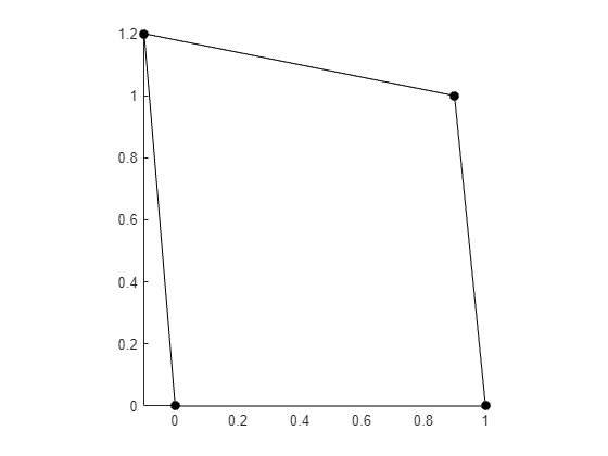

using $\bm \varphi \left(\xi ,\eta \right) \mathbf P = \left\lbrack x,y\right\rbrack$ and solving again for $\xi \left(x,y\right)$ and $\eta \left(x,y\right)$ we get the non-linear system of equations

syms x y xi eta
eqs = phi(xi, eta)*P == [x y];
eqs = simplify(eqs).'

notice how we can not formulate a system of the form $\mathbf A \xi + \mathbf B \eta +C=0$. We can, however, solve this equation system symbolically to get two solutions

[xi, eta] = solve(eqs,[xi,eta])

here, in the two solutions $\xi_1 \left(x,y\right)$ and $\xi_2 \left(x,y\right)$, only one is within the valid parametric space $\xi ,\eta \in \left\lbrack 0,1\right\rbrack$, which is $\xi_1$ and $\eta_1$ (after testing).

We can substitue the $\bm \varphi \left(\xi_1 ,\eta_1 \right)$ to get $\bm \varphi \left(x,y\right)$ which we can evaluate in all nodes, we should get the identiy matrix.

xi = xi(1); eta = eta(1);
phi_xy = matlabFunction(simplify(phi(xi,eta)))

phi_xy = 
    @(x,y)[x.*(-5.1e+1./2.0)-y.*5.0-sqrt(x.*-1.2e+1-y.*2.0+x.^2+3.6e+1).*(4.9e+1./2.0)+1.48e+2,x.*(6.1e+1./2.0)+y.*5.0+sqrt(x.*-1.2e+1-y.*2.0+x.^2+3.6e+1).*(5.9e+1./2.0)-1.77e+2,x.*-3.0e+1-y.*5.0-sqrt(x.*-1.2e+1-y.*2.0+x.^2+3.6e+1).*3.0e+1+1.8e+2,x.*2.5e+1+y.*5.0+sqrt(x.*-1.2e+1-y.*2.0+x.^2+3.6e+1).*2.5e+1-1.5e+2]

phi_xy(P(:,1),P(:,2))

ans = 4x4    
    1.0000         0         0         0
         0    1.0000         0         0
    0.0000         0    1.0000         0
         0         0         0    1.0000

Seems good! But note that, obviously, it is not efficient to have to deal with solving a non-linear system. Which is why we prefer to work in the parametric space if we can!

For our problem where we want to generate the function $u_h \left(x,y\right)$, we can now use $u_h \left(x,y\right)=\bm \varphi \left(x,y\right) \bf U$

syms x y
Uh(x,y) = phi_xy(x,y)*U

Uh(0,0) = 20

Now to visualize the interpolated field, it is again much easier to to do in the parametric space, i.e.,

N = 100;
xi = linspace(0,1,N);
eta = xi;
[Xi, Eta] = meshgrid(xi,eta);
UH = phi(Xi(:),Eta(:))*U;

PP = phi(Xi(:),Eta(:))*P;
X = reshape(PP(:,1),N,N);
Y = reshape(PP(:,2),N,N);
UH = reshape(UH,N,N);

figure; axis equal tight; hold on
surf(X,Y,Y*0,UH,'EdgeColor','none')
colormap jet; colorbar
contour(X,Y,UH,5,'EdgeColor','k')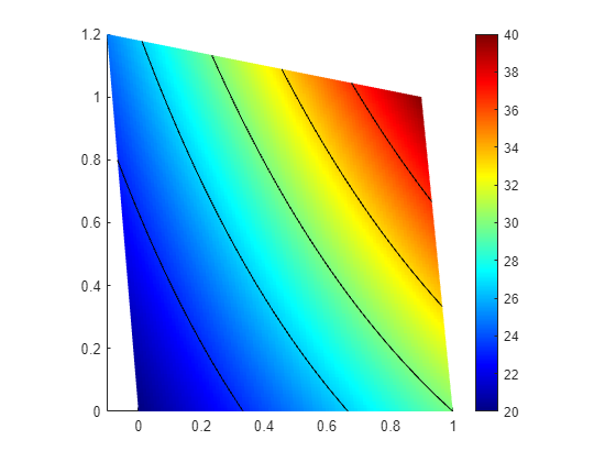

Here we can clearly see the curved (non-linear) nature of the bi-linear interpolant.