Download this page as a Matlab LiveScript
Table of contents
Iso-parametric mapping
We want to solve
\[ \begin{cases} -\dfrac{d^{2}u}{d\;x}+u=x & \text{for }x\in[1,5]\\ \\ \dfrac{du}{dx}\left(1\right)=-2,\ u\left(5\right)=1 \end{cases} \]The weak form of the DE is:
\[\int_1^5 \dfrac{d\;u}{d\;x}\dfrac{d\;v}{d\;x}d\;x+\int_1^5 u\;v\;d\;x{=\int_1^5 x\;v\;d\;x+\left\lbrack \dfrac{d\;u}{d\;x}v\right\rbrack }_1^5\]We will use approximate this using linear elements and insert the approximation into the weak form:
\[\int_1^5 \dfrac{d\;{\varphi }^T }{d\;x}u \dfrac{d\;{\varphi }^{\;} }{d\;x}d\;x+\int_1^5 {\varphi }^T u \;{\varphi }^{\;\;} d\;x=\int_1^5 x\;{\varphi }^T \;d\;x+{\left\lbrack \dfrac{d\;u}{d\;x}\varphi \right\rbrack }_1^5 \;\;\;\]We can break out \(u\) to get the system formulation
\[\left({\mathit{\mathbf{S} } }_{\;} +M_{\;} \right)u =f +g\]where the element stiffness matrix is
\[{ {\mathit{\mathbf{S} } }_e }_{\;} =\int_{x_1 }^{x_2 } \dfrac{d\;{\varphi }^T }{d\;x}\dfrac{d\;{\varphi }^{\;} }{d\;x}d\;x\]the mass matrix
\[{M_e }_{\;} =\int_{x_1 }^{x_2 } {\varphi }^T \;{\varphi }^{\;\;} d\;x\]and the element stiffness vector
\[{f_e }_{\;} =\int_{x_1 }^{x_2 } {\varphi }^T \;x\;d\;x\]We want to find a method to efficiently compute these integrals numerically, since currently we are computing them symbolically which is a very slow and inefficient way of utilizing computational power.
Consider the example element stiffness matrix below
\[{\mathit{\mathbf{S} } }_e =\int_{x_1 }^{x_2 } \dfrac{d\;{\varphi }^T }{d\;x}\dfrac{d\;\varphi }{d\;x}\mathrm{dx}\]This integral is in general hard (or very inefficient) to integrate for the general range \(x\in \left\lbrack x_1 ,x_2 \right\rbrack\). It would be easier if \(x\in \left\lbrack 0,1\right\rbrack\) (or \(x\in \left\lbrack -1,1\right\rbrack\)) always, for every element! That way we can apply smart integration rules as we shall see in the next lecture.
Using the parametric mapping we can switch from \(x\in \left\lbrack x_1 ,x_2 \right\rbrack\) to \(x\in \left\lbrack 0,1\right\rbrack\) for every element. The advantages are that the basis functions are the same for every element and that we can utilize numerical integration to compute the integrals. This makes the computations efficient and straight forward compared to the previous approach, where we had to define the basis functions for each element, compute the derivatives and integration symbolically. Remember, numerical methods are several orders of magnitude faster than symbolic. For industrial sized problems, we must implement the fastest method possible since these seconds quickly add upp to hours or even days for larger multidimensional problems!
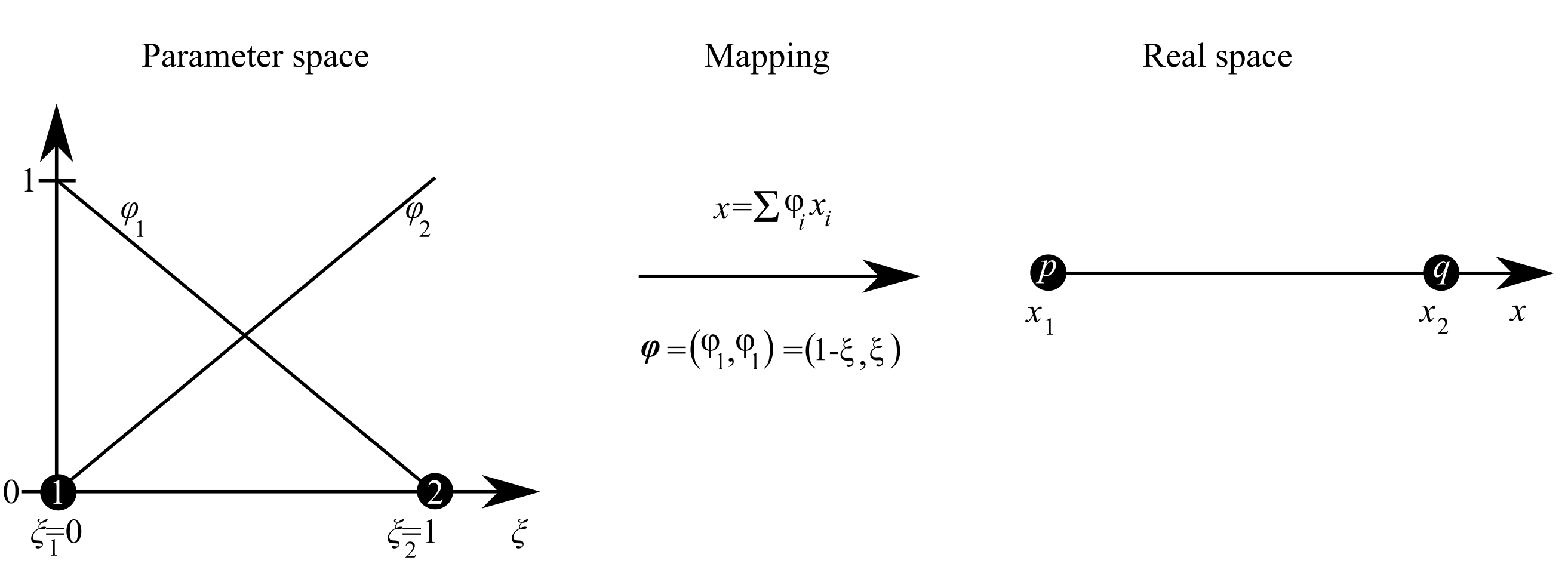
We can map from the parametric space to the real space using the basis functions defined in the parametric space, e.g., for linear elements in \(\xi \in \left\lbrack 0,1\right\rbrack\)
\[\varphi \left(\xi \right)=\left\lbrack 1-\xi ,\;\xi \right\rbrack\]So \(x\) defined on the interval \(x\in \left\lbrack x_1 ,x_2 \right\rbrack\) is given by
\[x=\sum_i \varphi_i \left(\xi \right)x_i =\left(1-\xi \right)x_1 +\xi \;x_2 =x_1 +\left(x_2 -x_1 \right)\xi\]so \(\left(\xi =0\Rightarrow x=x_1 ,\xi =1\Rightarrow x=x_2 \right)\)
and thus we have \(\varphi_i \left(x\left(\xi \right)\right)=\varphi_i \left(\xi \right)\), meaning that instead of using basis functions defined in the real space, we can instead use basis functions defined in the parametric space and thus our integration limits are the same every time!
But, we also need to define \(\frac{d\;\varphi }{d\;x}\) in the parametric space, which we can using the chain rule:
\[\dfrac{d\;\varphi_i }{d\;x}=\dfrac{d\;\varphi_i \left(\xi \right)}{d\;\xi }\;\dfrac{d\;\xi }{d\;x}\]Ok, \(\frac{d\;\varphi_i \left(\xi \right)}{d\;\xi }\;\;\) is straight forward, but what about \(\frac{d\;\xi }{d\;x}\)?
Well, the inverse is easy: \(\frac{d\;x}{d\;\xi }=\frac{d}{d\;\xi}\left(x_1 +\left(x_2 -x_1 \right)\xi \right)=\underset{\Delta x}{\underbrace{x_2 -x_1 } } =:h\)
in 1D, \(\frac{d\;x}{d\;\xi }\) this is the mesh/element size, \(h\), but it is also known as the Jacobian (Jacobian matrix, since in 2D and 3D it becomes a matrix as we will see in later lectures).
So we can get
\[\dfrac{d\;\varphi_i }{d\;x}=\dfrac{d\;\varphi_i \left(\xi \right)}{d\;\xi }\;\dfrac{d\;\xi }{d\;x}=\dfrac{d\;\varphi_i \left(\xi \right)}{d\;\xi }\;\dfrac{1}{h}=\dfrac{d\;\varphi_i \left(\xi \right)}{d\;\xi }\;J^{-1}\]We can also derive \(d\;x\)
\[\dfrac{d\;x}{d\;\xi }=h\Rightarrow d\;x=h\;d\xi\]which will be useful for integration. Generally \(\frac{d\;x}{d\;\xi }\) can be computed by
\(\frac{d\;x}{d\;\xi }=\sum_i \frac{d\;\varphi_i \left(\xi \right)}{d\;\xi }x_i\) which is easily computed since it only depends on the element coordinates \(x_i\).
We can now formulate the weak expression in the parametric domain:
\[\left(\int_1^5 \dfrac{d\;{\varphi }^T }{d\;x}\dfrac{d\;{\varphi }^{\;} }{d\;x}d\;x+\int_1^5 {\varphi }^T \;{\varphi }^{\;\;} d\;x\right)u =\int_1^5 {\varphi }^T \cdot x\;d\;x+\underset{g }{\underbrace{ {\left\lbrack \dfrac{d\;u}{d\;x}\varphi \right\rbrack }_1^5 \;\;\;} }\] \[=\left(\int_0^1 {\dfrac{d\;\underline{\varphi_{\xi } } }{d\;\xi } }^T \dfrac{1}{h}\dfrac{d\;\underline{\varphi_{\xi } } }{d\;x}\dfrac{1}{h}h\;d\;\xi +\int_0^1 {\varphi }^T \varphi \;h\;d\;\xi \right)u_e =\int_0^1 {\varphi }^T \cdot x\;h\;d\xi +g\] \[=\left(\underset{ {\mathit{\mathbf{S}} }_e }{\underbrace{\int_0^1 \frac{d\;{\underline{\varphi} }^T }{d\;\xi }\frac{d\;\underline{\varphi} }{d\;\xi }\frac{1}{h}\;d\;\xi } } +\underset{ {\mathit{\mathbf{M}} }_e }{\underbrace{\int_0^1 {\underline{\varphi} }^T \underline{\varphi} \;h\;d\;\xi } } \right)\underline{u_e } =\underset{f_e }{\underbrace{\int_0^1 {\underline{\varphi} }^T \cdot x\;h\;d\xi } } +\underline{g}\]Please note how we dropped the subindex in \(\varphi_{\xi }\) in order to make notation easier. We know which basis function is meant (the basis function defined in parametric space or real space) by the the context in which it is used.
We can use the same basis functions in all elements, the only thing that changes is the mesh size. This means that almost everything can be precomputed outside of the main for-loop for efficiency.
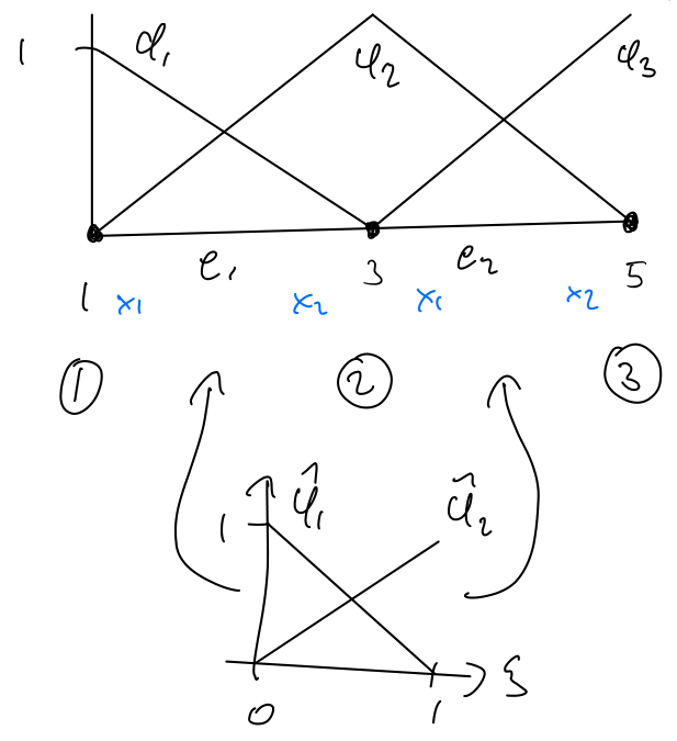
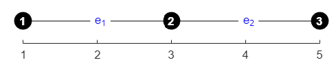
For every element we have \(\varphi =\left\lbrack \begin{array}{cc} 1-\xi & \xi \end{array}\right\rbrack\), \(\frac{d\;\varphi }{d\;x}=\left\lbrack \begin{array}{cc} -1 & 1 \end{array}\right\rbrack\)
Element 1: \(x_1 =1,x_2 =3\)
Plug everything into \({\mathit{\mathbf{S} } }_e\) and \({\mathit{\mathbf{M} } }_e\)
\[ \def\arraystretch{2.5} \begin{align*} \boldsymbol{S}_{e}^{1} & =\int_{1}^{3}\dfrac{d\varphi}{dx}^{T}\dfrac{d\varphi}{dx}dx\overset{\mathrm{Iso}-\mathrm{Parametric}\;\mathrm{map}}{=}\int_{0}^{1}\dfrac{d\varphi}{dx}^{T}\dfrac{d\varphi}{dx}h_{1}d\xi\\ & =\int_{0}^{1}\dfrac{d\varphi}{d\xi}^{T}\dfrac{1}{h_{1}}\dfrac{d\varphi}{d\xi}\dfrac{1}{h_{1}}h_{1}d\xi\\ & =\int_{0}^{1}\dfrac{d\varphi}{d\xi}^{T}\dfrac{d\varphi}{d\xi}\dfrac{1}{h_{1}}d\xi \end{align*} \] \[ \def\arraystretch{1} \begin{align*} & =\int_0^1 {\left\lbrack \begin{array}{c} -1\\ 1 \end{array}\right\rbrack }_{2\times 1} {\left\lbrack \begin{array}{cc} -1 & 1 \end{array}\right\rbrack }_{1\times 2} \dfrac{1}{h_1 }d\xi =\int_0^1 \left\lbrack \begin{array}{cc} 1 & -1\\ -1 & 1 \end{array}\right\rbrack \dfrac{1}{h_1 }d\xi \\ & =\left\lbrack \begin{array}{cc} 1 & -1\\ -1 & 1 \end{array}\right\rbrack \dfrac{1}{h_1 }=\left\lbrack \begin{array}{cc} 1 & -1\\ -1 & 1 \end{array}\right\rbrack \dfrac{1}{x_2 -x_1 } \end{align*} \]and for the element mass matrix for element 1
\[ \begin{align*} \boldsymbol M_e^1 & = \int_1^3 {\varphi }^T \varphi \;d\;x\overset{\mathrm{Iso}-\mathrm{Parametric}\;\mathrm{map} }{=} \int_0^1 {\varphi }^T \varphi {\;h}_1 d\xi\\ \end{align*} \] \[ \begin{align*} & =\int_0^1 \left\lbrack \begin{array}{c} 1-\xi \\ \xi \end{array}\right\rbrack \left\lbrack \begin{array}{cc} 1-\xi & \xi \end{array}\right\rbrack \;h_1 d\xi =\int_0^1 \left\lbrack \begin{array}{cc} 1-2\xi +\xi^2 & \xi -\xi^2 \\ \xi -\xi^2 & \xi^2 \end{array}\right\rbrack h_1 d\xi\\ &=\left\lbrack \begin{array}{cc} 1/3 & 1/6\\ 1/6 & 1/3 \end{array}\right\rbrack h_1 =\left\lbrack \begin{array}{cc} 1/3 & 1/6\\ 1/6 & 1/3 \end{array}\right\rbrack x_2 -x_1 \end{align*} \]the element load vector for element 1:
\[f_e^1 =\int_1^3 {\varphi }^T \cdot x\;d\;x\overset{\mathrm{Iso}-\mathrm{Parametric}\;\mathrm{map} }{=} \int_0^1 {\varphi }^T x\;h_{\;1} \;d\xi\]now, since we have \(f\left(x\right)=x\;\)we need to use the iso-parametric map on it: \(x=\sum_i \varphi_i x_i =\varphi \cdot {x }_c =\varphi \cdot \left\lbrack \begin{array}{c} x_1 \\ x_2 \end{array}\right\rbrack =x_2 \xi -x_1 \left(\xi -1\right)\)
thus we get for \(x_1=1\) and \(x_2=3\) \(x\left(\xi \right) = 1+2\xi\)
\[f_e^1 =\int_0^1 {\varphi }^T \;\left(\varphi \cdot \left\lbrack \begin{array}{c} x_1 \\ x_2 \end{array}\right\rbrack \right)h_1 \;d\xi =\int_0^1 \left\lbrack \begin{array}{c} 1-\xi \\ \xi \end{array}\right\rbrack \left(1+2\xi \right)h_1 d\xi\] \[ \def\arraystretch{1.5} f_e^1 =\int_0^1 \left\lbrack \begin{array}{c} -{\left(2\xi+1\right)}\,{\left(\xi-1\right)}\\ \xi \,{\left(2\xi+1\right)} \end{array}\right\rbrack h_1 d\xi =\left\lbrack \begin{array}{c} \frac{5}{2}\\ \frac{7}{3} \end{array}\right\rbrack \]Element 2: \(x_1 =3,{\;x}_2 =5\)
\[h_2 =x_2 -x_1 =2=h_1\]Note that if the elements are evenly spaced (or have the same aspect ratio in general) we get that the element stiffness and mass matrices are the same for every element and thus \({\mathit{\mathbf{S} } }_e^2 ={\mathit{\mathbf{S} } }_e^1\) and \({\mathit{\mathbf{M} } }_e^2 ={\mathit{\mathbf{M} } }_e^2\)
The load vector however is unique for every element since \(f\left(x\right)\;\)is different for every element in our case.
\[f_e^2 =\int_0^1 {\varphi }^T \;\left(\varphi \cdot \left\lbrack \begin{array}{c} x_1 =3\\ x_2 =5 \end{array}\right\rbrack \right)h_2 \;d\xi =\int_0^1 \left\lbrack \begin{array}{c} 1-\xi \\ \xi \end{array}\right\rbrack \left(3+2\xi \right)h_2 d\xi\] \[ \def\arraystretch{1.5} f_e^2 =\left\lbrack \begin{array}{c} \frac{11}{3}\\ \frac{13}{3} \end{array}\right\rbrack \]The mesh:
And the same process applies for the mass matrix, \(\mathit{\mathbf{M} }\)
Since \({\mathit{\mathbf{S} } }_e^i =\left\lbrack \begin{array}{cc} 1 & -1\\ -1 & 1 \end{array}\right\rbrack \frac{1}{h_i }\) we get
\[\mathit{\mathbf{S} }=\dfrac{1}{h}\left\lbrack \begin{array}{ccc} 1 & -1 & 0\\ -1 & 2 & -1\\ 0 & -1 & 1 \end{array}\right\rbrack \overset{\mathrm{with}\;h=2}{=} \left\lbrack \begin{array}{ccc} 1/2 & -1/2 & 0\\ -1/2 & 1 & -1/2\\ 0 & -1/2 & 1/2 \end{array}\right\rbrack\]and with \({\mathit{\mathbf{M} } }_e^i =\left\lbrack \begin{array}{cc} 1/3 & 1/6\\ 1/6 & 1/3 \end{array}\right\rbrack h_i\) we get the mass matrix
\[\mathit{\mathbf{M} }=h\left\lbrack \begin{array}{ccc} 1/3 & 1/6 & 0\\ & 2/3 & 1/6\\ \mathrm{sym} & & 1/3 \end{array}\right\rbrack \overset{\mathrm{with}\;h=2}{=} \left\lbrack \begin{array}{ccc} 2/3 & 1/3 & 0\\ 1/3 & 4/3 & 1/3\\ 0 & 1/3 & 2/3 \end{array}\right\rbrack\]finally the load vector
\[ \def\arraystretch{1.5} f\left(\left\lbrack 1,2\right\rbrack \right)=f\left(\left\lbrack 1,2\right\rbrack \right)+f_e^1 =\left\lbrack \begin{array}{c} \frac{7}{24}\\ \frac{1}{3}\\ 0 \end{array}\right\rbrack \] \[ \def\arraystretch{1.5} f\left(\left\lbrack 2,3\right\rbrack \right)=f\left\lbrack 2,3\right\rbrack +f_e^2 =\left\lbrack \begin{array}{c} \frac{7}{24}\\ \frac{1}{3}+\frac{5}{12}\\ \frac{11}{24} \end{array}\right\rbrack =\left\lbrack \begin{array}{c} \frac{7}{24}\\ \frac{3}{4}\\ \frac{11}{24} \end{array}\right\rbrack \]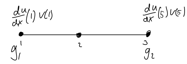
We combine the stiffness matrix and mass matrix into one system matrix
\[\mathit{\mathbf{S} }=\left(\mathit{\mathbf{S} }+\mathit{\mathbf{M} }\right)\]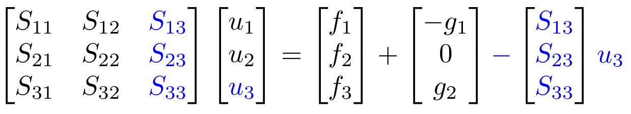
Since \(u_3\) is known and not 0, it will affect the system, it is acting as a reaction force and needs to be treated as such. We multiply the column corresponding to this degree of freedom and move it to the right hand side.
\[\left\lbrack \begin{array}{ccc} S_{11} & S_{12} & S_{13} \\ S_{21} & S_{22} & S_{23} \\ S_{31} & S_{32} & S_{33} \end{array}\right\rbrack \left\lbrack \begin{array}{c} u_1 \\ u_2 \\ u_3 \end{array}\right\rbrack =\left\lbrack \begin{array}{c} f_1 \\ f_2 \\ f_3 \end{array}\right\rbrack +\left\lbrack \begin{array}{c} -g_1 \\ 0\\ g_2 \end{array}\right\rbrack -\left\lbrack \begin{array}{c} S_{13} u_3 \\ S_{23} u_3 \\ S_{33} u_3 \end{array}\right\rbrack\]We are then reducing the system by removing equations where \(u\) is known!
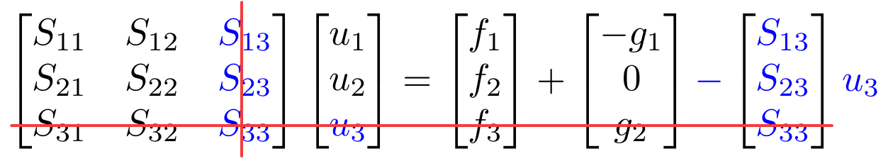
The free degrees of freedom are thus 1 and 2 and our equation system becomes
\[\left\lbrack \begin{array}{cc} S_{11} & S_{12} \\ S_{21} & S_{22} \end{array}\right\rbrack \left\lbrack \begin{array}{c} u_1 \\ u_2 \end{array}\right\rbrack =\left\lbrack \begin{array}{c} f_1 \\ f_2 \end{array}\right\rbrack +\left\lbrack \begin{array}{c} -g_1 \\ 0 \end{array}\right\rbrack -\left\lbrack \begin{array}{c} S_{13} u_3 \\ S_{23} u_3 \end{array}\right\rbrack\] \[ \def\arraystretch{1.5} \left\lbrack \begin{array}{c} u_1 \\ u_2 \end{array}\right\rbrack ={\left\lbrack \begin{array}{cc} S_{11} & S_{12} \\ S_{21} & S_{22} \end{array}\right\rbrack }^{-1} \left\lbrack \begin{array}{c} f_1 -g_1 -S_{13} u_3 \\ f_2 -S_{23} u_3 \end{array}\right\rbrack =\left\lbrack \begin{array}{c} \frac{345}{97}\\ \frac{281}{97} \end{array}\right\rbrack \]clear
N = 2;
xnod = linspace(1,5,N+1);
nodes = [(1:N)', (2:N+1)'];
nnod = length(xnod);
neq = nnod*1;
S = zeros(neq,neq);
M = S;
f = zeros(neq,1);
syms xi
phi = [1-xi, xi];
dphi = [-1, 1];
for iel = 1:N
iel
inods = nodes(iel, :);
xc = xnod(inods);
x1 = xc(1); x2 = xc(2);
h = x2-x1;
Se = int(dphi'*dphi*1/h, xi, 0, 1)
Me = int(phi'*phi*h, xi, 0, 1)
x = phi*[x1;x2]
fe = int(phi.'*x*h, xi, 0, 1)
S(inods,inods) = S(inods, inods) + Se
M(inods,inods) = M(inods, inods) + Me
f(inods) = f(inods) + fe
end
S = S+Miel = 1S = 3x3
0.5000 -0.5000 0
-0.5000 0.5000 0
0 0 0
M = 3x3
0.6667 0.3333 0
0.3333 0.6667 0
0 0 0
f = 3x1
1.6667
2.3333
0
iel = 2S = 3x3
0.5000 -0.5000 0
-0.5000 1.0000 -0.5000
0 -0.5000 0.5000
M = 3x3
0.6667 0.3333 0
0.3333 1.3333 0.3333
0 0.3333 0.6667
f = 3x1
1.6667
6.0000
4.3333S = 3x3
1.1667 -0.1667 0
-0.1667 2.3333 -0.1667
0 -0.1667 1.1667Boundary conditions
\[\dfrac{d\;u}{d\;x}\left(1\right)=-2\Rightarrow g_1 = -2 \] \[u\left(5\right)=1\Rightarrow u_3 =1\]u = 3x1
0
0
1free = 1x2
1 2g = 3x1
2
0
0F = 3x1
3.6667
6.1667
3.1667Solve for the free degrees of freedom
u = 3x1
    3.5567
    2.8969
1.0000sym(u)Visualize
\[ \begin{cases} -\dfrac{d^{2}u}{dx^{2}}+u=x & \text{for }x\in[1,5]\\ \\ \dfrac{du}{dx}\left(1\right)=-2,\ u\left(5\right)=1 \end{cases} \]syms ue(x)
DE = -diff(ue,x,2)+ue==x;
du(x) = diff(ue,x,1);
BC = [du(1) == -2, ue(5) == 1];
ue(x) = dsolve(DE,BC)figure
fplot(ue,[1,5],'Color','r','LineWidth',2,'Displayname','Exact solution')
hold on
plot(xnod, u,'o-b','Displayname','Approximation')
title(sprintf('Approximation using %d linear elements',N))
legend show