PiecewiseFunctionApproximation

Download this page as a Matlab LiveScript

Table of contents

Approximating a function using piecewise elements
Matlab implementation of a piecewise linear approximation
\(L_2\) error measure
Error convergence study

Approximating a function using piecewise elements

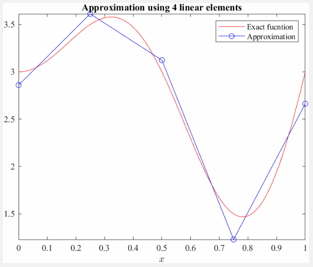
So we want to approximate the function

\[u\left(x\right)=2x\;\sin \left(2\pi x\right)+3\;\textrm{for}\;x\in \left\lbrack 0,1\right\rbrack\]

using piecewise elements of order 1 or 2.

This means finding all nodal values \(u_i\) to the approximation (the blue circles in the figure above). This problem can be formulated using Galerkin as such: Find \(u_i\) such that

\[\int_{0}^{1}r(x,u_{i})\varphi_{i}dx=0\] \[=\int_0^1 \left(U\left(x,u_i\right) - u\left(x\right)\right)\varphi_j \;d\;x\;=0\]

with \(U\left(x,u_i\right)=\sum_i \varphi_i \left(x\right){u}_i\)

Now, this is the same old Galerkin expression as we had in the previous section. In order to apply a piecewise approximation, we shall further expand the expressions to formulate a matrix system!

Expanding the expression in the integral we get

\[\int_0^1 \left(\sum_i \varphi_i \left(x\right)\varphi_j \left(x\right){\;u}_i -u\left(x\right)\varphi_j \left(x\right)\right)\;d\;x\;=0\] \[=\int_0^1 \sum_i \varphi_i \left(x\right)\varphi_j \left(x\right){\;u}_i \;d\;x-\int_0^1 u\left(x\right)\varphi_j \left(x\right)\;d\;x=0\]

move \(u_i \;\)out

\[\sum_i \int_0^1 \varphi_i \left(x\right)\varphi_j \left(x\right)\;d\;x\;\;{\;u}_i =\int_0^1 u\left(x\right)\varphi_j \left(x\right)\;d\;x\]

which is equivalent to the matrix system

\(M_{\textrm{ij} } u_i =f_i\) or \(\mathit{\mathbf{M} }\;\mathit{\mathbf{u} }=\mathit{\mathbf{f} }\)

Solving this system gets us all nodal values for \(u_i\).

Piecewise approximation - The mesh

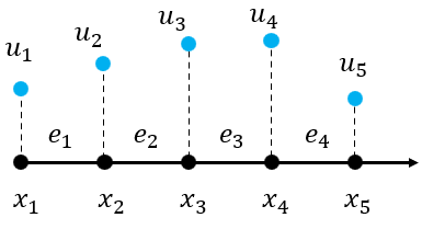
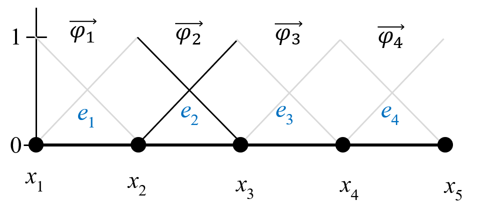
To describe any mesh we need a coordinate matrix (vector in 1D)

\[ \mathbf{x}=\begin{bmatrix}x_{1}\\ x_{2}\\ x_{3}\\ x_{4}\\ x_{5} \end{bmatrix} \]

and a nodal connectivity matrix

\[ \mathbf{T}=\begin{bmatrix}1 & 2\\ 2 & 3\\ 3 & 4\\ 4 & 5 \end{bmatrix} \]

4 linear elements will lead to 5 equations to be solved for \(u_i ,i=1,2,\ldotp \ldotp \ldotp ,5\)

\[ \mathbf{u}=\begin{bmatrix}u_{1}\\ u_{2}\\ u_{3}\\ u_{4}\\ u_{5} \end{bmatrix} \]

An element \(e\) between nodes \(x_i\) and \(x_j\) contributes only to equations \(i\;\)and \(j\). We can use the \(e\)'th row of \(\mathbf T\) to see which nodes are associated with the element \(e\).

Example: Element mass matrix for element 3 between node 3 and 4:

\[\begin{array}{l} \;\;\;\;\begin{array}{ccccc} \;1 & \;2 & \;\;3 & \;\;\;4 & \;\;5 \end{array}\\ \begin{array}{c} 1\\ 2\\ 3\\ 4\\ 5 \end{array}\underset{\mathit{\mathbf{M}}}{\underbrace{\left\lbrack \begin{array}{ccccc} & & & & \\ & & & & \\ & & M_{33} & M_{34} & \\ & & M_{43} & M_{44} & \\ & & & & \end{array}\right\rbrack } } \end{array}\]

\[ \def\arraystretch{2.5} \begin{array}{l} M_{33} =\int_{x_3 }^{x_4 } \varphi_3 \varphi_3 dx\\ M_{34} =\int_{x_3 }^{x_4 } \varphi_3 \varphi_4 dx\\ M_{43} =\int_{x_3 }^{x_4 } \varphi_4 \varphi_3 dx\\ M_{44} =\int_{x_3 }^{x_4 } \varphi_4 \varphi_4 dx\\ \end{array} \]

Local Numbering

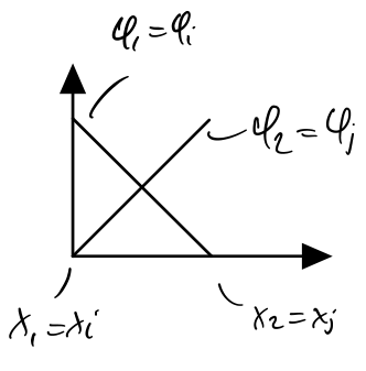
We can use local node numbering to simplify things:

Now, for each element \(e\) we define \(x_1\) and \(x_2\), compute \(\varphi\) and then compute \(\mathbf{M}^e\) and \(\mathbf{f}^e\)

Element stiffness matrix

\[\mathbf{M}^e =\int_{x_1 }^{x_2 } \boldsymbol\varphi^T \boldsymbol\varphi dx\]

\[ \def\arraystretch{2.5} \mathbf{M}^{e}=\begin{bmatrix}\int_{x_{1}}^{x_{2}}\varphi_{1}\varphi_{1} \;dx & \int_{x_{1}}^{x_{2}}\varphi_{1}\varphi_{2} \;dx\\ \int_{x_{1}}^{x_{2}}\varphi_{2}\varphi_{1} \;dx & \int_{x_{1}}^{x_{2}}\varphi_{2}\varphi_{2} \;dx \end{bmatrix} \]

and element load vector

\[\mathbf{f}^e =\int_{x_1 }^{x_2 } \varphi^T u(x) \;dx\]

\[ \def\arraystretch{2.0} \mathbf{f}^e =\left\lbrack \begin{array}{c} \int_{x_1 }^{x_2 } u(x) \varphi_1 \;dx\\ \int_{x_1 }^{x_2 } u(x) \varphi_2 \;dx \end{array}\right\rbrack \]

Utilizing a piecewise approximation leads to the element mass matrix and element load vector:

\[M_e =\int_{x_1 }^{x_2 } {\varphi }^T \varphi \;d\;x\]

and

\[f_e =\int_{x_1 }^{x_2 } {\varphi }^T u\left(x\right)\;d\;x\]

which need to be assembled into the global mass matrix and load vectors.

Assembly process

For each element \(e\), we add \(\mathbf{M}^e\) and \(\mathbf{f}^e\) to the correct place in \(\mathbf{M}\) and \(\mathbf{f}\).

Element 1: M([1,2],[1,2])

Element 2: M([2,3],[2,3])

Element 3: M([3,4],[3,4])

Element 4: M([4,5],[4,5])

We need to add each element contribution to the global mass matrix.

\[\begin{array}{l} M_{\textrm{ii}}^{\textrm{new}} = M_{\textrm{ii}}^{\textrm{old}} + M_{11}^e \\ M_{\textrm{ij}}^{\textrm{new}} = M_{\textrm{ij}}^{\textrm{old}} + M_{12}^e \\ \vdots \end{array}\]

\[\begin{array}{l} f_i^{\textrm{new}} =f_i^{\textrm{old}} +f_1^e \\ f_j^{\textrm{new}} =f_j^{\textrm{old}} +f_2^e \end{array}\]

or on matrix form

\[ M(\text{row},\text{col}) \]

where row denotes the array containing the row indices and col the column indices. Thus we could write

\[ M([i,j],[i,j]) \]

to mean a sub-matrix of \(M\) with rows \(i\) and \(j\) and columns \(i\) and \(j\).

The corresponding Matlab (or Julia) syntax is

M([i,j],[i,j]) = M([i,j],[i,j]) + Me

All nodes that have several elements will get contributions from each element. We are "accumulating" mass to these nodes from the elements.

Contribution from element 1

\[{\mathit{\mathbf{M}}\left(\left\lbrack 1,2\right\rbrack ,\left\lbrack 1,2\right\rbrack \right)}_{2\times 2} ={\mathit{\mathbf{M}}\left(\left\lbrack 1,2\right\rbrack ,\left\lbrack 1,2\right\rbrack \right)}_{2\times 2} +M_{2\times 2}^{e_1 }\]

\[\begin{array}{l} \;\;\;\;\begin{array}{ccccc} \;\;\;\;\;1 & \;\;\;2 & 3 & 4 & 5 \end{array}\\ \begin{array}{c} 1\\ 2\\ 3\\ 4\\ 5 \end{array}\left\lbrack \begin{array}{ccccc} M_{11}^1 & M_{12}^1 & & & \\ M_{21}^1 & M_{22}^1 & & & \\ & & & & \\ & & & & \\ & & & & \end{array}\right\rbrack \end{array}\]

Contribution from element 2

\[{\mathit{\mathbf{M}}\left(\left\lbrack 2,3\right\rbrack ,\left\lbrack 2,3\right\rbrack \right)}_{2\times 2} ={\mathit{\mathbf{M}}\left(\left\lbrack 2,3\right\rbrack ,\left\lbrack 2,3\right\rbrack \right)}_{2\times 2} +M_{\;}^{e_2 }\]

\[\begin{array}{l} \;\;\;\;\begin{array}{ccccc} \;\;\;\;\;1 & \;\;\;\;\;\;\;\;2 & \;\;\;\;\;\;\;\;3 & 4 & 5 \end{array}\\ \begin{array}{c} 1\\ 2\\ 3\\ 4\\ 5 \end{array}\left\lbrack \begin{array}{ccccc} M_{11}^1 & M_{12}^1 & & & \\ M_{21}^1 & M_{22}^1 +M_{11}^2 & M_{12}^2 & & \\ & M_{21}^2 & M_{22}^2 & & \\ & & & & \\ & & & & \end{array}\right\rbrack \end{array}\]

etc

For four linear elements, this leads to the equation system

\[ \left(\begin{array}{c} 0.083\,u_1 +0.042\,u_2 =0.39\\ 0.042\,u_1 +0.17\,u_2 +0.042\,u_3 =0.85\\ 0.042\,u_2 +0.17\,u_3 +0.042\,u_4 =0.72\\ 0.042\,u_3 +0.17\,u_4 +0.042\,u_5 =0.45\\ 0.042\,u_4 +0.083\,u_5 =0.27 \end{array}\right) \]

Solving the linear system

We end up with the linear system of equations

\[ \mathbf{Mu=f} \]

which is solved by using a linear equations solver, in Matlab we do this by

u = M\f

We will do this in code now using linear element and symbolic integration.

Matlab implementation of a piecewise linear approximation

clear

syms x
ue(x) = 2*x*sin(2*pi*x)+3;

N = 4;
nnod = N+1;
xnod = linspace(0,1,N+1);
nodes = [(1:nnod-1)', (2:nnod)'];

Phi = @(x,x1,x2) [(x2-x)/(x2-x1), (x-x1)/(x2-x1)];

M = zeros(nnod,nnod); F = zeros(nnod,1);
for iel = 1:N
    inod = nodes(iel,:);
    xc = xnod(inod);
    x1 = xc(1); x2 = xc(2);
    phi = @(x)Phi(x,x1, x2);

    Me = int(phi(x).'*phi(x), x,x1,x2);
    fe = int(phi(x).'*ue(x), x,x1,x2);
    
    M(inod,inod) = M(inod,inod) + Me;
    F(inod) = F(inod) + fe;
end

u = M\F;

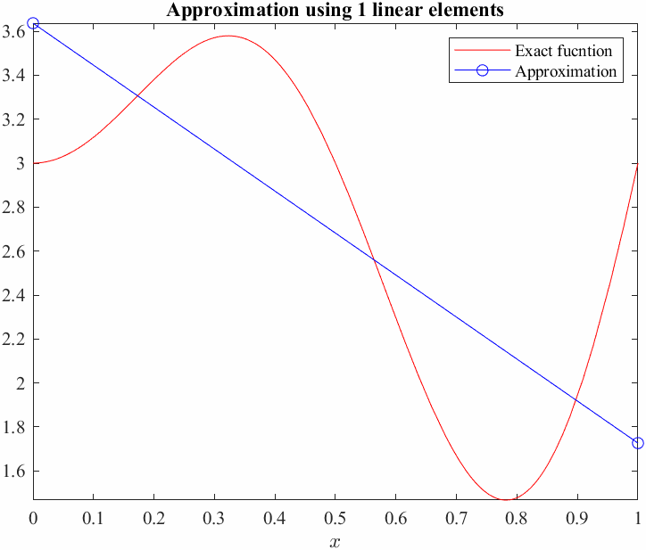
figure
fplot(ue,[0,1],'r','LineWidth',2); hold on
plot(xnod,u,'-bo')

\(L_2\) error measure

Now, we will compute the average error between the exact function and our Galerkin approximation, we shall use the \(L_2\) norm as a measure of error. This basicaly means squaring the difference between the functions over the entire domain and taking the square root.

\[L_2 \textrm{error}:=\sqrt{\int_0^1 {\left(U-u\right)}^2 \;d\;x}\]

So we need to compute the difference between the function for each element and adding it all up.

\[L_2 \textrm{error}:=\sqrt{\int_0^1 {\left(U-u\right)}^2 \;d\;x}=\sqrt{\sum_e^N \int_e^{\;} {\left(U_e -u\right)}^2 \;d\;x}\]

where

\[U_e \left(x\right)=\varphi \left(x\right){\mathit{\mathbf{u} } }_e \overset{\textrm{lin}\;\textrm{ele} }{=} \left\lbrack \begin{array}{cc} \varphi_1 & \varphi_1 \end{array}\right\rbrack \left\lbrack \begin{array}{c} u_1 \\ u_2 \end{array}\right\rbrack\]

L2err = 0;
for iel = 1:N
    inod = nodes(iel,:);
    x1 = xnod(inod(1)); x2 = xnod(inod(2));
    phi = @(x)Phi(x,x1, x2);
    U = phi(x)*u(inod);
    L2err = L2err + double(int((U-ue)^2, x,x1,x2));
end
L2err = sqrt(L2err)

L2err = 0.1106

Error convergence study

Now we can start changing \(N\) to see how the error goes down. If we plot \(N\) versus the error we get a convergence plot.

Linear approximation

clear
syms x
ue(x) = 2*x*sin(2*pi*x)+3;

NN = [2,4,8,16,32];
L2Err = [];
Time = [];

figure
fplot(ue,[0,1],'r','LineWidth',2); hold on
hp = plot(NaN,NaN,'-b.');

for N = NN
    tic
    nnod = N+1;
    xnod = linspace(0,1,N+1);
    nodes = [(1:nnod-1)', (2:nnod)'];
    
    Phi = @(x,x1,x2) [(x2-x)/(x2-x1), (x-x1)/(x2-x1)];
    
    M = zeros(nnod,nnod); F = zeros(nnod,1);
    for iel = 1:N
        inod = nodes(iel,:);
        xc = xnod(inod);
        x1 = xc(1); x2 = xc(2);
        phi = @(x)Phi(x,x1, x2);
    
        Me = vpaintegral(phi(x).'*phi(x), x,x1,x2);
        fe = vpaintegral(phi(x).'*ue(x), x,x1,x2);
        
        M(inod,inod) = M(inod,inod) + Me;
        F(inod) = F(inod) + fe;
    end
    
    u = M\F;
    t1 = toc;
    Time(end+1) = t1;

    L2err = 0;
    for iel = 1:N
        inod = nodes(iel,:);
        x1 = xnod(inod(1)); x2 = xnod(inod(2));
        phi = @(x)Phi(x,x1, x2);
        U = phi(x)*u(inod);
        L2err = L2err + double(vpaintegral((U-ue)^2, x,x1,x2));
    end
    L2err = sqrt(L2err);

    L2Err(end+1) = L2err;

    set(hp,'XData',xnod, 'YData',u);
    title(sprintf("Approximation using %d linear elements",N))
    pause(0.1)
    drawnow
end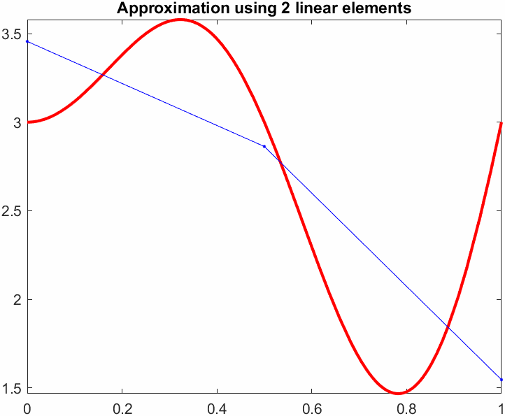

Quadratic approximation

syms x1 x2 x3 x
A = [1 x1 x1^2
     1 x2 x2^2
     1 x3 x3^2];
C = A\eye(3);
Phi = simplify([1 x x^2]*C);
Phi = matlabFunction(Phi);

Time2 = []; L2Err2 = [];

figure;
for N = NN
    tic
    nnod = N*2+1;
    xnod = linspace(0,1,nnod);
    nodes = [(1:2:nnod-2)', (2:2:nnod-1)', (3:2:nnod)'];
    neq = nnod*1;
    
    M = zeros(nnod,nnod); F = zeros(nnod,1);
    for iel = 1:N
        inod = nodes(iel,:);
        xc = xnod(inod);
        x1 = xc(1); x2 = xc(2); x3 = xc(3);
        phi = @(x)Phi(x,x1, x2, x3);
    
        Me = vpaintegral(phi(x).'*phi(x), x,x1,x3);
        fe = vpaintegral(phi(x).'*ue(x), x,x1,x3);
    
        M(inod,inod) = M(inod,inod) + Me;
        F(inod) = F(inod) + fe;
    end
    
    u = M\F;
    t1 = toc;
    Time2(end+1) = t1;
    
    L2err = 0;
    for iel = 1:N
        inod = nodes(iel,:);
        xc = xnod(inod);
        x1 = xc(1); x2 = xc(2); x3 = xc(3);
        phi = @(x)Phi(x,x1, x2, x3);
        U = phi(x)*u(inod);
        L2err = L2err + double(vpaintegral((U-ue)^2, x,x1,x3));
    end
    L2err = sqrt(L2err);
    L2Err2(end+1) = L2err;
    
    
    clf
    fplot(ue,[0,1],'r','LineWidth',1); 
    hold on
    
    for iel = 1:N
        inod = nodes(iel,:);
        xc = xnod(inod);
        x1 = xc(1); x2 = xc(2); x3 = xc(3);
        phi = @(x)Phi(x,x1, x2, x3);
        U = phi(x)*u(inod);
    
        fplot(U, [x1,x3])
        plot(xc,u(inod),'.b');
    end
    title(sprintf("Approximation using %d quadratic elements",N))
%     if N == 2
%         exportgraphics(gca,"PiecewiseQuadratic.gif","Append",false)
%     end
%     for i = 1:10
%         exportgraphics(gca,"PiecewiseQuadratic.gif","Append",true)
%     end
end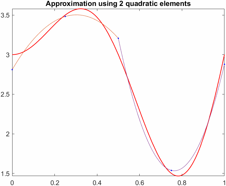

Error convergence graphs

figure; hold on
plot(NN,L2Err,'-ko','DisplayName','Linear')
plot(NN,L2Err2,'-ks','DisplayName','Quadratic')
set(gca,'xscale','log','yscale','log')
xlabel("N"); ylabel("L_2 error")
xticks(NN)
xticklabels({'2','4','8','16','32'})
grid on
legend show

Note how the quadratic approximation not only has a lower initial error but also a steeper slope, meaning it converges faster.

figure; hold on
plot(NN,Time,'-ko','DisplayName','Linear')
plot(NN,Time2,'-ks','DisplayName','Quadratic')
set(gca,'xscale','log','yscale','log')
xlabel("N"); ylabel("Time (s)")
xticks(NN)
xticklabels({'2','4','8','16','32'})
yticks([0.5,1,2,4,8,16])
grid on
legend("show",location="northwest")