Table of contents
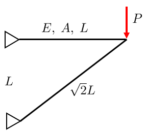
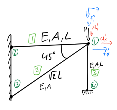
The simple truss is represented by two rods that are attached to each other in the right corner (node) using a pin connector which is assumed to be moment free. The other two ends of the rods are firmly fixed in place, which is denoted by the two triangles. A point force is placed at the node, denoted by \(P\). The rods can only carry axial force, meaning that loads cannot be applied anywhere but at the nodes. This problem is a 2D planar problem, so every node has two degrees of freedom i.e., it can be translated in the \(x\) and \(y\)-direction.
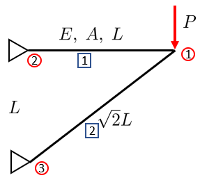
We begin our analysis by numbering each rod and each node. Each rod has four quantities of interest: normal forces, \(N_i\), normal stresses, \(\sigma_i\), strains, \(\varepsilon_i\) and deformations \(\delta_i\) where \(i=1,2\). Additionally each node has two quantities of interest: nodal forces \(f_j\) and nodal displacements \(u_j\) where \(j=1,2,3\).
For a structure like this, the interesting questions are:
Is the structure able to carry the load? The the structural requirements are typically posed on the maximum stress and displacements as well as reaction forces, i.e., nodal forces at the boundary conditions.
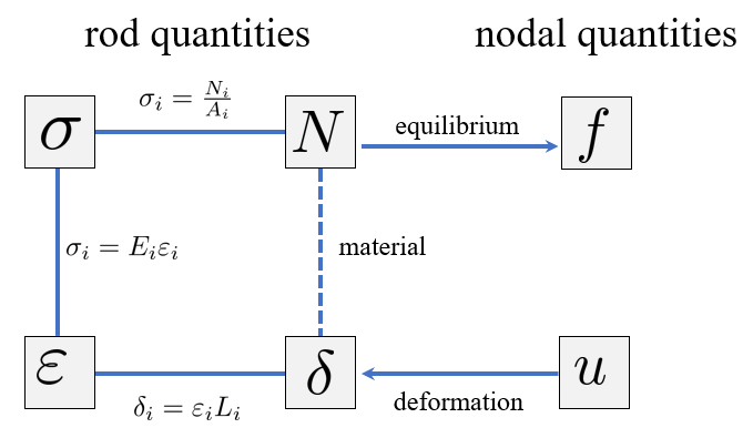
An overview of the relations between nodal quantities and rod quantities is given by the figure below
These relations essentially form the equation
\[ \delta=\dfrac{FL}{EA} \]which is the simplest solution (setting \(f=0\)) to the boundary value problem:
\[ \boxed{ \text{BVP}\begin{cases} -\dfrac{d}{dx}\left(EA\dfrac{du}{dx}\right)=f & \text{for }x\in[0,L]\\ u(0)=L\\ EA\dfrac{du}{dx}(L)=F \end{cases} } \]This is why the method in this (and the following) section is also known as the direct approach, since we are tackling the differential equation directly, but also with a loss of generality.
In what follows, we shall derive a method for determining the displacements \(u\) of all nodes given a set of external forces \(f\).
For our problem, we can see that we have four boundary conditions: \(u_2^x =u_2^y =u_3^x =u_3^y =0\). The known nodal loads are \(f_1^y =-P\). Furthermore we know the rod quantities \(E_1 =E_2 =E\), \(A_1 =A_2 =A\), \(L_1 =L\) and \(L_2 =\sqrt{2}L\).
We want to know the displacements in node 1, the reaction forces in nodes, 2 and 3 and all rod normal forces, stresses, strains and deformations.
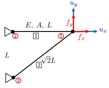
The node 1 is said to be free, i.e., able to be translated in \(x\) and \(y\). We say that node 1 has two degrees of freedom.
We now introduce the displacement field (vector) which corresponds to each degree of freedom.
\[ \def\arraystretch{1.5} \bm u=\left\lbrack \begin{array}{c} u_1^x \\ u_1^y \end{array}\right\rbrack \]Additionally, we introduce the nodal load vector
\[ \def\arraystretch{1.5} \bm f =\left\lbrack \begin{array}{c} f_1^x \\ f_1^y \end{array}\right\rbrack \]We will replace the known loads later, i.e., we will evaluate \(f_1^y =-P\) at a later time.
The problem is to find a relation between the loads \(\bm f\) and the displacements \(\bm u\). This is done by computing the stiffness matrix for the structure such that
\[\boldsymbol S \boldsymbol u = \bm f \Rightarrow \boldsymbol u = \boldsymbol S^{-1} \bm f \]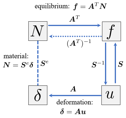
Equilibrium of an isolated node leads to the matrix \({\mathit{\mathbf{A} } }^T\) directly, this approach is known as method of joints.
Setting up material relations leads to the \({\mathit{\mathbf{S} } }^e\) matrix directly.
Thus having \(\boldsymbol A^T\) and \(\boldsymbol S^e\) gives
\[\boldsymbol S = \boldsymbol A^T \boldsymbol S^e \boldsymbol A \Rightarrow \boldsymbol u = \boldsymbol S^{-1} \bm f \]Once the displacements are known, we can compute the rod quantities:
\( \boldsymbol \delta = \boldsymbol A \boldsymbol u\), \(\boldsymbol N = \boldsymbol S^e \boldsymbol \delta\) and finally \(\sigma_i =N_i /A_i\)
Step 1: Number all rod and nodes
Step 2: Introduce a coordinate system
Step 3: Introduce the displacement vector and load vector
\[\mathit{\mathbf{u} }=\left\lbrack \begin{array}{c} u_1^x \\ u_1^y \end{array}\right\rbrack\] \[\mathit{\mathbf{f} }=\left\lbrack \begin{array}{c} f_1^x \\ f_1^y \end{array}\right\rbrack\]Step 4: Rod fields
\[\boldsymbol \delta =\left\lbrack \begin{array}{c} \delta_1 \\ \delta_2 \\ \delta_3 \end{array}\right\rbrack ,\mathit{\mathbf{N} }=\left\lbrack \begin{array}{c} N_1 \\ N_2 \\ N_3 \end{array}\right\rbrack\]Step 5: Determine either \({\mathit{\mathbf{A} } }^T\) by equilibrium using the method of joints or determine \(\mathit{\mathbf{A} }\) using the unit displacements method. We shall do both and you can decide what method you prefer.
Use the deformation relation
\[\boldsymbol \delta =\mathit{\mathbf{A} }\;\mathit{\mathbf{u} }\]first, set \(\mathit{\mathbf{u} }=\left\lbrack \begin{array}{c} 1\\ 0 \end{array}\right\rbrack :\)
\[\left\lbrack \begin{array}{c} \delta_1 \\ \delta_2 \\ \delta_3 \end{array}\right\rbrack =\left\lbrack \begin{array}{cc} A_{11} & A_{12} \\ A_{21} & A_{22} \\ A_{31} & A_{32} \end{array}\right\rbrack \left\lbrack \begin{array}{c} 1\\ 0 \end{array}\right\rbrack =\left\lbrack \begin{array}{c} A_{11} \\ A_{21} \\ A_{31} \end{array}\right\rbrack\]i.e., we get the first column of \(\mathit{\mathbf{A} }\), likewise, setting \(\mathit{\mathbf{u} }={\left\lbrack \begin{array}{cc} 0 & 1 \end{array}\right\rbrack }^T\) will give us the second column.
Now we apply this using a deformation figure
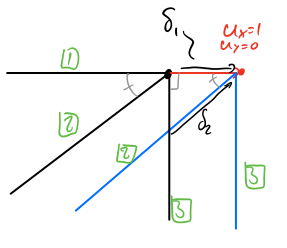
Assuming small deformations (small deformation theory) all rods must be only translated such that they stay parallell to each other.
We look at the deformation in the \(x\)-direction:
\[\begin{array}{l} \delta_1^x =1\\ \delta_2^x =\textrm{cos45}\degree =\dfrac{1}{\sqrt{2} }\\ \delta_3^x =0 \end{array}\]Now in the \(y\)-direction:
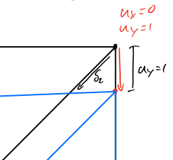
Note, here the deformation are negative, since we are compressing the rods.
These deformations lead to
\[\Rightarrow A=\left\lbrack \begin{array}{cc} \delta_1^x & \delta_1^y \\ \delta_2^x & \delta_2^y \\ \delta_3^x & \delta_3^y \end{array}\right\rbrack =\left\lbrack \begin{array}{cc} 1 & 0\\ \dfrac{1}{\sqrt{2} } & -\dfrac{1}{\sqrt{2} }\\ 0 & -1 \end{array}\right\rbrack\]This matrix is purely geometrically determined!
equilibrium of the node (joint):
Note: Be aware of the directions considering the coordinate system!
\[\begin{array}{l} \to :f_1^x -N_1 -N_2 \textrm{cos45}\degree =0\\ \downarrow :f_1^y +N_3 +N_2 \textrm{sin45}\degree =0 \end{array}\] \[\begin{array}{l} \Rightarrow f_1^x =N_1 +N_2 \dfrac{1}{\sqrt{2} }\\ f_1^y =-N_2 \dfrac{1}{\sqrt{2} }-N_3 \end{array}\]On matrix form:
\[\left\lbrack \begin{array}{c} f_1^x \\ f_1^y \end{array}\right\rbrack =\underset{ {\mathit{\mathbf{A} } }^T }{\underbrace{\left\lbrack \begin{array}{ccc} 1 & \dfrac{1}{\sqrt{2} } & 0\\ 0 & -\dfrac{1}{\sqrt{2} } & -1 \end{array}\right\rbrack } } \left\lbrack \begin{array}{c} N_1 \\ N_2 \\ N_3 \end{array}\right\rbrack\]Note: Determine either \(\mathit{\mathbf{A} }\) or \({\mathit{\mathbf{A} } }^T\) using which ever method you feel is easier and then just transpose!.
Step 6: Material relations, \(\mathit{\mathbf{N} }={\mathit{\mathbf{S} } }^e \boldsymbol \delta\)
For each rod we have
\[\delta_i =\dfrac{N_i L_i }{E_i A_i }\Rightarrow N_i =\dfrac{E_i A_i }{L_i }\delta_i\]or on matrix form
\[\left\lbrack \begin{array}{c} N_1 \\ N_2 \\ N_3 \end{array}\right\rbrack =\underset{ {\mathit{\mathbf{S} } }^e }{\underbrace{\left\lbrack \begin{array}{ccc} \frac{E_1 A_1 }{L_1 } & 0 & 0\\ 0 & \frac{E_2 A_2 }{L_2 } & 0\\ 0 & 0 & \frac{E_3 A_3 }{L_3 } \end{array}\right\rbrack } } \left\lbrack \begin{array}{c} \delta_1 \\ \delta_2 \\ \delta_3 \end{array}\right\rbrack\]or
\[\left\lbrack \begin{array}{c} N_1 \\ N_2 \\ N_3 \end{array}\right\rbrack =\underset{ {\mathit{\mathbf{S} } }^e }{\underbrace{\left\lbrack \begin{array}{ccc} \dfrac{E_1 A_1 }{L_1 } & \dfrac{E_2 A_2 }{L_2 } & \dfrac{E_3 A_3 }{L_3 } \end{array}\right\rbrack \odot \underset{\mathit{\mathbf{I} } }{\underbrace{\left\lbrack \begin{array}{ccc} 1 & 0 & 0\\ 0 & 1 & 0\\ 0 & 0 & 1 \end{array}\right\rbrack } } } } \left\lbrack \begin{array}{c} \delta_1 \\ \delta_2 \\ \delta_3 \end{array}\right\rbrack\]where \( \odot \) is the Hadamard product, i.e., element-wise multiplication. In Matlab this is written as A .* B.
\(E_1 =E_2 =E_3 =E\), \(A_1 =A_2 =A_3 =A\), \(L_1 =L_3 =L\) and \(L_2 =\sqrt{2}L\).
Leading to
\[{\Rightarrow \mathit{\mathbf{S} } }^e =\dfrac{E\;A}{L}\left\lbrack \begin{array}{ccc} 1 & 0 & 0\\ 0 & \dfrac{1}{\sqrt{2} } & 0\\ 0 & 0 & 1 \end{array}\right\rbrack\]Step 7: Put everything together
\[\mathit{\mathbf{f} }={\mathit{\mathbf{A} } }^T \mathit{\mathbf{N} }={\mathit{\mathbf{A} } }^T {\mathit{\mathbf{S} } }^e \boldsymbol \delta =\underset{\mathit{\mathbf{S} } }{\underbrace{ {\mathit{\mathbf{A} } }^T {\mathit{\mathbf{S} } }^e \mathit{\mathbf{A} } } } \;\mathit{\mathbf{u} }\] \[\Rightarrow \mathit{\mathbf{f} }=\mathit{\mathbf{S} }\;\mathit{\mathbf{u} }\] \[\begin{array}{l} S=\dfrac{E\;A}{L}\left\lbrack \begin{array}{ccc} 1 & \dfrac{1}{\sqrt{2} } & 0\\ 0 & -\dfrac{1}{\sqrt{2} } & -1 \end{array}\right\rbrack \left\lbrack \begin{array}{ccc} 1 & 0 & 0\\ 0 & \dfrac{1}{\sqrt{2} } & 0\\ 0 & 0 & 1 \end{array}\right\rbrack \left\lbrack \begin{array}{cc} 1 & 0\\ \dfrac{1}{\sqrt{2} } & -\dfrac{1}{\sqrt{2} }\\ 0 & -1 \end{array}\right\rbrack \\ =\dfrac{E\;A}{L}\left\lbrack \begin{array}{cc} 1+\dfrac{1}{2\sqrt{2} } & -\dfrac{1}{2\sqrt{2} }\\ -\dfrac{1}{2\sqrt{2} } & 1+\dfrac{1}{2\sqrt{2} } \end{array}\right\rbrack \end{array}\]Step 8: Apply known values on \(\mathit{\mathbf{f} }\) (and/ or \(\mathit{\mathbf{u} }\))
\[\mathit{\mathbf{f} }=\left\lbrack \begin{array}{c} 0\\ P \end{array}\right\rbrack =P\left\lbrack \begin{array}{c} 0\\ 1 \end{array}\right\rbrack\]solve the system: \(\mathit{\mathbf{u} }={\mathit{\mathbf{S} } }^{-1} \mathit{\mathbf{f} }=\left\lbrace \underset{\mathrm{S}\backslash \mathrm{f} }{\textrm{MATLAB} } \right\rbrace =\frac{P\;L}{E\;A}\left\lbrack \begin{array}{c} \frac{\sqrt{2} }{2\left(\sqrt{2}+2\right)}\\ -\left(\frac{\sqrt{2} }{2}-\frac{3}{2}\right) \end{array}\right\rbrack \approx \frac{P\;L}{E\;A}\left\lbrack \begin{array}{c} 0\ldotp 2071\\ 0\ldotp 7929 \end{array}\right\rbrack\)
Step 9: The rod forces, strains, deformations and stresses are computed using \(\mathit{\mathbf{u} }\)!
\[N={\mathit{\mathbf{S} } }^e \mathit{\mathbf{A} }\;\mathit{\mathbf{u} }\approx P\left\lbrack \begin{array}{c} 0\ldotp 2071\\ -0\ldotp 2929\\ -0\ldotp 7929 \end{array}\right\rbrack\]Note! In cases when \({\mathit{\mathbf{A} } }^T\) is square (static determinate structure) we can get the rod forces directly from the loads: \(\mathit{\mathbf{N} }={\left({\mathit{\mathbf{A} } }^T \right)}^{-1} \mathit{\mathbf{f} }\).
\[\boldsymbol \delta =\mathit{\mathbf{A} }\;\mathit{\mathbf{u} }\] \[\sigma_i =\dfrac{N_i }{A_i }\]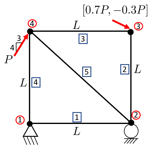
The boundary condition at node 1 means \(u_1^x =u_1^y =0\) and at node two, we have the boundary condition \(u_2^y =0\).
Determine the displacements, symbolically.
Set \(E=A=L=P=1\) and plot the displaced structure.
Modify the boundary condition at node 2 to be \(u_2^y =-\frac{1}{5}\frac{P\;L}{E\;A}\) and determine the rest of the displacements, plot!
Solution
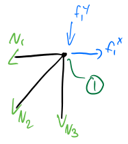
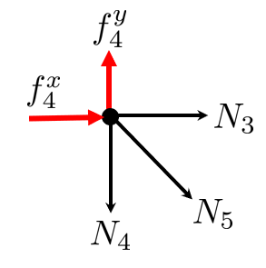
We start by posing equilibrium equations on nodes which are partly free, i.e., nodes 2, 3 and 4.
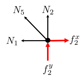
Node 2:
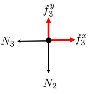
Node 3:
Node 4:
Note how we are skipping node 1, since all degrees of freedom are prescribed to zero. We could add it though, and deal with eliminating equations later.
Then we can combine the node equations
\[\left\lbrack \begin{array}{c} f_2^x \\ f_2^y \\ f_3^x \\ f_3^y \\ f_4^x \\ f_4^y \end{array}\right\rbrack =\left\lbrack \begin{array}{ccccc} 1 & 0 & 0 & 0 & 1/\sqrt{2}\\ 0 & -1 & 0 & 0 & -1/\sqrt{2}\\ 0 & 0 & 1 & 0 & 0\\ 0 & 1 & 0 & 0 & 0\\ 0 & 0 & -1 & 0 & -1/\sqrt{2}\\ 0 & 0 & 0 & 1 & 1/\sqrt{2} \end{array}\right\rbrack \left\lbrack \begin{array}{c} N_1 \\ N_2 \\ N_3 \\ N_4 \\ N_5 \end{array}\right\rbrack\]or
\[\mathit{\mathbf{f} }={\mathit{\mathbf{A} } }^T \mathit{\mathbf{N} }\]from which we identify \({\mathit{\mathbf{A} } }^T\).
Material relations
Here we formulate the lengths of the bars, each entry along the diagonal corresponds to a bar.
\[S^e =E\;A\left\lbrack \begin{array}{ccccc} \dfrac{1}{L} & 0 & 0 & 0 & 0\\ 0 & \dfrac{1}{L} & 0 & 0 & 0\\ 0 & 0 & \dfrac{1}{\;L} & 0 & 0\\ 0 & 0 & 0 & \dfrac{1}{\;L} & 0\\ 0 & 0 & 0 & 0 & \dfrac{1}{\sqrt{2}L} \end{array}\right\rbrack\]or
\[{\mathit{\mathbf{S} } }^e =E\;A\;\left\lbrack \dfrac{1}{L},\dfrac{1}{L},\dfrac{1}{L},\dfrac{1}{L},\dfrac{1}{\sqrt{2}L}\right\rbrack \odot \mathit{\mathbf{I} }\]Stiffness matrix
\[\mathit{\mathbf{S} }={\mathit{\mathbf{A} } }^T {\mathit{\mathbf{S} } }^e \mathit{\mathbf{A} }\]Now we will implement this using Matlab since it's kindof cumbersome to solve a \(6\times 6\) system by hand.
syms E A L P
sq = 1/sqrt(2);
AT = [1   0   0    0   sq
      0  -1   0    0  -sq
      0   0   1    0    0
      0   1   0    0    0
      0   0  -1    0   -sq
      0   0   0    1    sq];
Se = E*A*[1/L 1/L 1/L 1/L sq*1/L] .* eye(5);
S = AT*Se*AT'Now we insert what we know into the system.
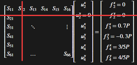
\[ \def\arraystretch{1.5} \left\lbrack \begin{array}{cccccc} S_{11} & S_{12} & S_{13} & S_{14} & S_{15} & S_{16} \\ S_{21} & & & & & \\ S_{31} & & \ddots & & & \vdots \\ S_{41} & & & & & \\ S_{51} & & & & & \\ S_{61} & & \ldots & & & S_{66} \end{array}\right\rbrack \left\lbrack \begin{array}{c} u_2^x \\ u_2^y =0\\ u_3^x \\ u_3^y \\ u_4^x \\ u_4^y \end{array}\right\rbrack =\left\lbrack \begin{array}{c} f_2^x =0\\ f_2^y =0\\ f_3^x =0\ldotp 7P\\ f_3^y =-0\ldotp 3P\\ f_4^x =3/5P\\ f_4^y =4/5P \end{array}\right\rbrack \]We have to reduce the system, by removing equations where the solution \(u\) is known. This means, deleting row 2 and column 2.
f = [0
     0
     0.7*P
     0.3*P
     3/5*P
     4/5*P];
u = sym(zeros(6,1));
presc = 2;
free = [1,3,4,5,6];
u(free) = S(free,free)\f(free)Visualization
In order to visualize the displacements, we need numeric data, in this case, we were not provided with data, so we set everything to 1.
E = 1; A = 1; L = 1; P = 1;
u = double(subs(u))
u = 6x1
1.3000
0
7.7770
0.3000
7.0770
2.1000We split the x and y components of the displacements into a matrix with the first column being the x-components and the second column being the y-components.
U = [0 0
     u(1:2:end), u(2:2:end)]
U = 4x2
0 0
1.3000 0
7.7770 0.3000
7.0770 2.1000Now, we shall create the topology of the structure, first the coordinates of our structure:
p = [0 0
     L 0
     L L
     0 L];
Then the edge connectivity.
edges = [1 2
         2 3
         3 4
         1 4
         2 4];
Now we can send this off to the patch function, which draws the whole structure in one simple line.
figure
patch('Faces',edges,'Vertices',p,'LineWidth',2)
axis equal
hold on
Now we shall overlay the undeformed structure with our deformed structure. We do this by adding the displacement field to our coordinate field such that
\[P_{\textrm{deformed} } =P_{\textrm{undeformed} } +U\;s\]where we need to scale the displacement field such that it shows the trend without being overly deformed.
scale = 0.05;
patch('Faces',edges,'Vertices',p+U*scale,'LineWidth',1,'LineStyle',':')
Lastly, we add node numbering and edge numbering.
plot(p(:,1),p(:,2),'ok','MarkerFaceColor','c','MarkerSize',14)
text(p(:,1)-0.01,p(:,2),cellstr(num2str([1:4]')))
for i=1:5
    inod = edges(i,:);
    xm = mean(p(inod,1));
    ym = mean(p(inod,2));
    text(xm,ym,num2str(i),'backgroundColor','y')
end
We start by converting previously symbolic variables to numeric.
S = double(subs(S));
f = double(subs(f));
Modify the boundary condition at node 2 to be \(u_2^y =-\frac{1}{5}\frac{P\;L}{E\;A}\) and determine the rest of the displacements, plot! }
In this case, the displacement \(u_2^y\) is not zero, and causes a reaction force which affects the whole structure. We deal with this by modifying the right hand side. In other words, we need to subtract the reaction forces which this displacement causes from the load vector. The reaction force is
\[F_R =u_2^y \left\lbrack \begin{array}{c} S_{21} \\ S_{22} \\ S_{23} \\ S_{24} \\ S_{25} \\ S_{26} \end{array}\right\rbrack\]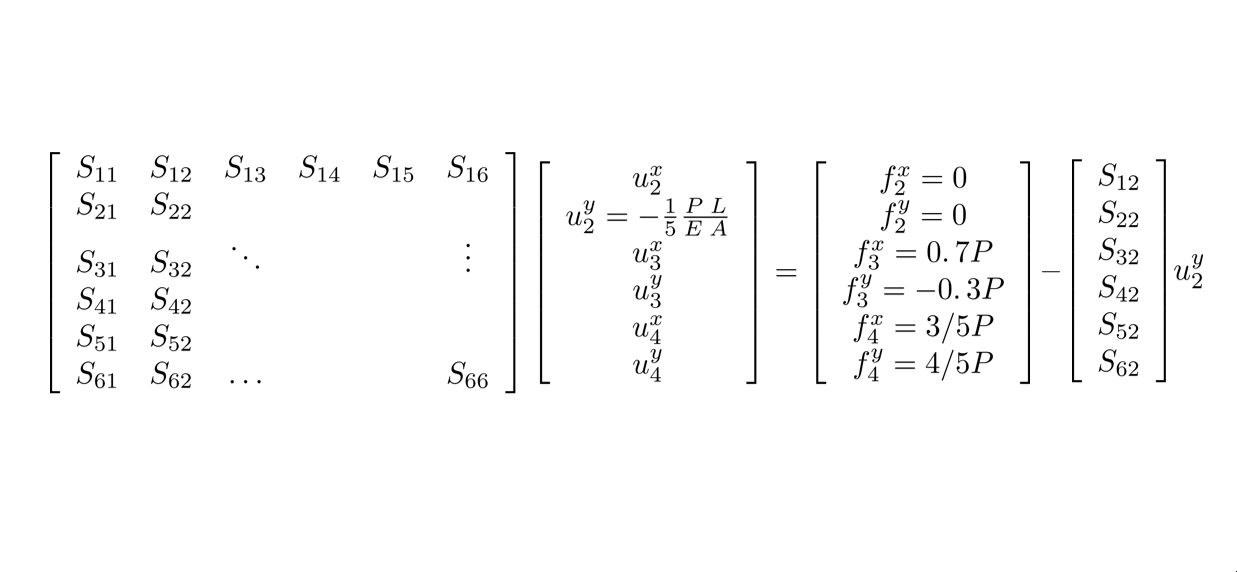
We end up with the reduced system of equations.
\[\left\lbrack \begin{array}{ccccc} S_{11} & S_{13} & S_{14} & S_{15} & S_{16} \\ S_{31} & \ddots & & & \vdots \\ S_{41} & & & & \\ S_{51} & & & & \\ S_{61} & \ldots & & & S_{66} \end{array}\right\rbrack \left\lbrack \begin{array}{c} u_2^x \\ u_3^x \\ u_3^y \\ u_4^x \\ u_4^y \end{array}\right\rbrack =\left\lbrack \begin{array}{c} f_2^x =0\\ f_3^x =0\ldotp 7P\\ f_3^y =-0\ldotp 3P\\ f_4^x =3/5P\\ f_4^y =4/5P \end{array}\right\rbrack -u_2^y \left\lbrack \begin{array}{c} S_{21} \\ S_{23} \\ S_{24} \\ S_{25} \\ S_{26} \end{array}\right\rbrack\]We do this in Matlab by defining a variable for the prescribed degree of freedom.
presc = 2;Then we modify the right-hand side
u = zeros(6,1);
u(presc) = -1/5*P*L/(E*A)
u = 6x1
0
-0.2000
0
0
0
0fr = S(:,presc)*u(presc)fr = 6x1
0.0707
-0.2707
0
0.2000
-0.0707
0.0707f = f - frf = 6x1
-0.0707
0.2707
0.7000
0.1000
0.6707
0.7293free = [1,3,4,5,6]; %Free degrees of freedom
S(free,free)ans = 5x5
1.3536 0 0 -0.3536 0.3536
0 1.0000 0 -1.0000 0
0 0 1.0000 0 0
-0.3536 -1.0000 0 1.3536 -0.3536
0.3536 0 0 -0.3536 1.3536f(free)ans = 5x1
-0.0707
0.7000
0.1000
0.6707
0.7293Now we solve the for the free DOFs.
u(free) = S(free,free)\f(free)u = 6x1
1.3000
-0.2000
7.9770
0.1000
7.2770
2.1000Now, let's visualize!
U = [0 0
     u(1:2:end), u(2:2:end)]
U = 4x2
0 0
1.3000 -0.2000
7.9770 0.1000
7.2770 2.1000figure
patch('Faces',edges,'Vertices',p,'LineWidth',2)
axis equal
hold on
scale = 0.05;
patch('Faces',edges,'Vertices',p+U*scale,'LineWidth',1,'LineStyle',':')
plot(p(:,1),p(:,2),'ok','MarkerFaceColor','c','MarkerSize',14)
text(p(:,1)-0.01,p(:,2),cellstr(num2str([1:4]')))
for i=1:5
inod = edges(i,:);
xm = mean(p(inod,1));
ym = mean(p(inod,2));
text(xm,ym,num2str(i),'backgroundColor','y')
end
We can see a rather small displacement in the negative y-direction in node 2. Comparing the numerical values shows that all displacements are displaced slightly downward.