Download this page as a Matlab LiveScript
Table of contents
The purpose of this initial work package is to get you up and running with computational thinking.
Since we are going to explore numerical methods such as the Finite Element Method, we need to be somewhat familiar with technical programming. Currently at JTH and in this course we have access to Matlab which will simplify implementations a lot.
Create the symbolic functions \(y\left(x\right)=3\;\sin \left(x\right)\) and \(g\left(x\right)=4\cos \left(2x\right)\) for \(x\in \left\lbrack -2\pi ,2\pi \right\rbrack\). Plot the functions and their derivatives in the same figure. Use x- and y-labels, titles, legend to clearly describe the four graphs.
Let
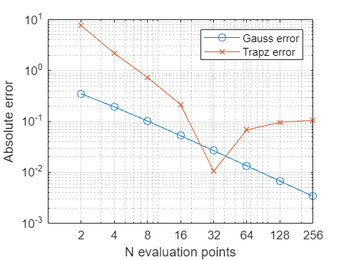
err_G = [0.3494 0.1937 0.1025 0.0528 0.0268 0.0135 0.0068 0.0034];
err_Trapz = [7.6100 2.1818 0.7381 0.2152 0.0106 0.0684 0.0968 0.1060];
NP = [2 4 8 16 32 64 128 256];
Plot the data in the two variables err_G and err_Trapz on the y-axis and NP on the x-axis. The the x- and y-scale to logarithmic. Change the graphical properties to achieve this figure:
Use symbolic variables and let
\[{\mathbf{S}}^e =\dfrac{E\;A}{L}\left\lbrack \begin{array}{ccc} 1 & 0 & 0\\ 0 & \dfrac{1}{\sqrt{2}} & 0\\ 0 & 0 & 1 \end{array}\right\rbrack\] \[{\mathbf{A}}^T =\left\lbrack \begin{array}{ccc} 1 & \dfrac{1}{\sqrt{2}} & 0\\ 0 & -\dfrac{1}{\sqrt{2}} & -1 \end{array}\right\rbrack\] \[\mathbf{f}=\left\lbrack \begin{array}{c} 0\\ P \end{array}\right\rbrack\]compute \(\mathbf{S}={\mathbf{A}}^T {\mathbf{S}}^e \mathbf{A}\) and \(\mathbf{u}={\mathbf{S}}^{-1} \mathbf{f}\), answer using decimal form and 4 significant numbers.
A ship is at the point A relative to the origin, given below.
Plot the vector \(\overrightarrow{\textrm{OA}} =\left\lbrack 3,1\right\rbrack\) using both quiver() and plot().
The ship needs to make a 90-degree counter-clockwise rotation from its current heading and sail 5 length units, this defines its position B. Plot this point. How far away from the origin is the ship?
Use a rotational matrix to rotate any amount and plot the point C by making a right turn of 30 degrees and sail 3 units from B.
Plot the routes O-A-B-C as straight lines.
Plot the joints as circles and add a small text box next to these usingtext() with the coordinates using one decimal precision.