The partial differential equation for the static linear elasticity problem
−∇⋅σ=fσ=2με+λI∇⋅uu=gσ⋅n=tin Ωin Ωon ∂ΩDon ∂ΩN
By multiplying (1) with a test function v and integrating by parts, see here, we end up with the weak form of the linear elasticity equation, which states: Find the displacement field u, with u=g on the boundary ∂ΩD, such that
∫Ωσ(u):ε(v)dΩ=∫Ωf⋅vdΩ+∫∂Ωt⋅vds∀v that are 0 on ∂ΩD
1: Partially discretized domain using linear triangles.
The weak form of the linear elasticity problem is posed on a domain Ω which needs to be discretized (meshed). This means dividing the domain into a finite amount of elements such that the problem can be tackled numerically, see Figure 1. In this section we will discuss this discretization and the choice of the weight function v using the Galerkin method [2] for the 2D linear elasticity problem, but the reader is also referred to the Galerkin Method section for more information. For completeness we shall give a brief introduction to the method here.
The Galerkin method belongs to a family of weighted residual methods. Consider a differential equation of the form
−dx2d2ku(x)=f(x) for x∈[a,b]
where enough boundary conditions are given such that a unique solution can exist, e.g., u(a)=0 and du/dx(b)=0. Now, an approximation method aims at solving (3). This is done by multiplying (3) by an arbitrary function v(x) (the weight function) to obtain
v(f+kdx2d2u)
This can be integrated over the domain of interest
−∫abdx2d2uvdx=∫abfvdx
See here for an in-depth explanation of the reasons for integrating the equation. Integrating the term with the higher order derivative by parts leads to the weak form:
∫abkdxdudxdvdx=∫abfvdx
In what follows we will not (yet) use the weak form, but just the integral form of the differential equation multiplied by the weight function to keep things general.
The solution to the differential equation can be approximated by a linear combination of some known functions φ(x) and unknown parameters ai:
u(x)≈U(x)=i=1∑naiφi(x)
where a1,...,an are unknown parameters and φ1(x),...,φn(x) are pre-specified functions, called trial or basis functions. The problem becomes to find these parameters a1,...,an which is done by substituting u(x) by U(x) in (5), which leads to the weighted residual method,
∫ab(dx2d2U(x)+f)vdx=0
with U(x) not satisfying the equation exactly in general, we get a residual
r(x)=dx2d2U(x)+f=0
which can be written as
∫abr(x)vdx=0
meaning that for a certain choice of v determines the unknowns a1,...,an and thus the approximating solution U(x) by minimizing the signed integral. Let v be a general function and constructed as a series of n linear combinations of known functions Vj(x) and arbitrary parameters cj such that
v(x)=V1c1+V2c2+...+Vncn=j∑Vjcj
Since the weight functions are arbitrary and Vj(x) are known, it must be concluded that cj are arbitrary and moreover, since cj are not depended on x we can pull them out of the integral and get
j∑cj∫abrVjdx=0
since this should hold for arbitrary cj we conclude that the following must hold
∫abrVjdx=0
which in fact is a series of n equations of the form
∫abrV1dx∫abrV2dx⋯∫abrVndx=0=0=0
substituting the approximation into the integral we get
∫ab(i=1∑ndx2d2φiai+f)Vjdx=0
where ai is not dependent on x and thus can be pulled out of the integral, leading to the n-by-n system
The procedure leading from the differential equation multiplied by the weight function to the system of equations is known as the weighted residual method and specific methods are obtained by making a choice of the weight function v, e.g., the least squares method where v=∂ai∂r, but the most popular one for the FEM is the Galerkin method. See Chapter 8 in [1] for more information.
Galerkin suggested that given that the trial function or approximation has the form U(x)=∑i=1naiφi(x), the weight function v should have the same form as the trial function, i.e., v(x)=∑i=1nciφi(x), meaning we should simply choose the basis functions as the weight functions, thus the Galerkin method takes the form:
∫abrφjdx=0
and loosely speaking, setting Vj=φj, and in the case of the weak form the derivative of the basis weight function become dxdVj=dxdφj such that the weak form in (5) becomes:
∫abkdxdUdxdφjdx=∫abfφjdx
and substituting the approximation gives
∫abk(i=1∑ndxdφiai)dxdφjdx=∫abfφjdx
which after pulling out ai of the integral, we get j=1,...,n equations:
In the previous section, Galerkin's method has only been discussed for approximations that are defined on the whole interval and also continuous on the whole interval. Since the first use was at a time where computers were not digital yet, the problems were kept small and the approximations simple. However, with the advent of the first digital computers came the use of Galerkin's method with piecewise polynomials which constitutes the finite element method.
To define a Galerkin Finite Element method for the elasticity problem in (2), we must introduce a finite dimensional subspaceVh, i.e., a set of piece-wise integrable functions, typically polynomials of low order (which translate to linear or quadratic triangle elements in 2D)
u(x,y)≈U(x,y)=i∑φi(x,y)ui
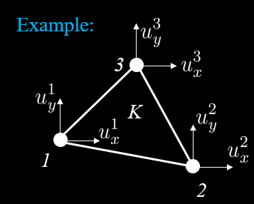
so that the functions φi constitute a base for Vh, i.e., any v∈Vh can be written as a linear combination of the basis functions φi as discussed in the previous section. The interpolation points at (xi,yi), ui=2D(uxiuyi)T are the nodal displacement vectors and make up the interpolant of u. The discrete displacement field for an n-noded mesh is represented by the displacement vector u=[ux1uy1ux2uy2⋯uxnuyn]T. This defines our discrete solution field on our mesh. We will in later sections take a look at the construction of elements and basis functions. Suffice to say for now we choose the basis functions, φi to have a local support, meaning they have the value φi=1 in the node i and φi=0 in all other nodes of the mesh. Thus ui has the value u in node i. The value of u between the nodes is interpolated using the basis function and we shall discuss the choice of polynomial order and its consequence on the approximation later.
As a first example: For a linear triangle, K, in 2D the displacement field takes the form uK=[ux1uy1ux2uy2ux3uy3]T.
The displacement field on element K is approximated using the interpolant, expressed on Voigt form using basis functions.
The B matrix contains spatial derivatives of the basis function of our element. We shall see in the next section how the basis functions can be derived for any element and in the section after that how the derivatives are derived and computed.
With these definitions, the matrix formulation corresponding to the FEM formulation of (1) becomes
we have ε:ε=εM⋅εM and λtrεI:ε can be written λ∇⋅uI:ε
∇⋅u=[∂x∂∂y∂][uxuy]
for which the corresponding discrete system is given by
Bdiv:=[∂x∂φ1∂y∂φ1∂x∂φ2∂y∂φ2⋯]
Using the Mandel notation, the discrete system becomes
(∫Ω2μBεTBε+λBdivTBdivdΩ)u=∫ΩΦTfdΩ+∫∂ΩΦTtds
Note that the linear system is the same both in the Voigt and Mandel form, however there are some benefits with the Mandel form. The expression is kept in the general form of the Hooke's Law. The expression is separated into the volumetric and deviatoric terms, which facilitates special treatment of integration known as hourglass control.
We have (using the Mandel notation), the element stiffness matrix
SK=∫K(2μBεTBε+λBDBD)dK
the element load vector
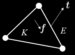
fK=∫KΦTf(x)dK
the traction (external force) vector
gE=∫EΦETt(x)dE
where E denotes edge (in 2D, where as in 3D it would be a surface). The edge element is one spatial dimension lower, we are formulating the equations on an edge instead of a triangle. For the edge element we have
N.
S. Ottosen and H. Petersson, Introduction to the finite element
method. New York etc.: Prentice Hall, 1992, pp. xv + 410.
[2]
B.
G. Galerkin, “Series occurring in various questions concerning the
elastic equilibrium of rods and plates,”Vestnik Inzhenerov i
Tekhnikov, (Engineers and Technologists Bulletin), vol. Vol. 19,
pp. 897–908, 1915.